A Programmable Look-Up Table-Based Interpolator with Nonuniform Sampling Scheme
Abstract
Interpolation is a useful technique for storage of complex functions on limited memory space: some few sampling values are stored on a memory bank, and the function values in between are calculated by interpolation. This paper presents a programmable Look-Up Table-based interpolator, which uses a reconfigurable nonuniform sampling scheme: the sampled points are not uniformly spaced. Their distribution can also be reconfigured to minimize the approximation error on specific portions of the interpolated function’s domain. Switching from one set of configuration parameters to another set, selected on the fly from a variety of precomputed parameters, and using different sampling schemes allow for the interpolation of a plethora of functions, achieving memory saving and minimum approximation error. As a study case, the proposed interpolator was used as the core of a programmable noise generator—output signals drawn from different Probability Density Functions were produced for testing FPGA implementations of chaotic encryption algorithms. As a result of the proposed method, the interpolation of a specific transformation function on a Gaussian noise generator reduced the memory usage to 2.71% when compared to the traditional uniform sampling scheme method, while keeping the approximation error below a threshold equal to 0.000030518.
1. Introduction
Nowadays, the world is facing a boom on the fusion between telecommunications and information technology. The merging of these two fields spreads over all kinds of information systems, requiring efforts for ensuring the integration among many kinds of organizations [1], from tactical to strategic operations, in different levels of information system interoperability [2]. The ISO/OSI seven-layer model arises as a lighthouse for seeking the interoperability on many different layers of networked solutions [3]. Many standards and protocols arise from this model, including cryptographic ones.
Encryption solutions can be implemented on both software and hardware. Software implementations are more related to the protection of the information itself, while hardware ones can be also used to protect the communication channels [4]. In the case of tactical telecommunication systems, which require both channel and information security, the hardware implementation of such encryption algorithms arises as a better compromise. The need to test the behavior of such systems against different sources of noise and jamming becomes the motivation to implement, on FPGA (Field-Programmable Gate Array), a programmable noise generator.
A Look-Up Table- (LUT-) based interpolation system is the core of the programmable noise generator developed in this work. Using a LUT, complex and otherwise slow calculations can be sped up by storing precomputed values of the function, interpolating the desired values in between, achieving high-speed designs [5]. Look-Up Tables are very common microelectronic blocks for many applications [5–19]. Ba et al. [9] proposed a linearly interpolated LUT predistorter used to mitigate the effects of nonlinear amplifiers. Monga and Bala [10] proposed an algorithm for minimizing the approximation error on multidimensional LUTs where both samples values and distributions are optimized.
Some authors used nonuniform sampling schemes as a solution for minimizing the LUT memory size: Seidner [11] reduced the memory usage on the implementation of a 10Y conversion circuit with a LUT scaling sample scheme; Yan and Mämmelä [15] used a nonuniformly segmented interpolation LUT for simulating nonlinear radio frequency power amplifiers; Cavers [16] proposed a systematic way to describe and analyze arbitrary nonuniform LUT sampling schemes as a companding function, which was further improved by Hassani and Kamarei [17] with a LUT segmentation concept; Boumaiza et al. [18] proposed a new companding function for amplifier predistortion with built-in dependence on the nonlinearity of the power amplifier; Dutra et al. [19] used a nonuniform but fixed sampling scheme to minimize the memory size of a LUT-based interpolator designed to represent the Inverse Error Function (erf−1).
All works previously mentioned used a fixed, uniform or not, sampling scheme to characterize a given function or class of functions. The main contribution of this work is to implement on FPGA a LUT-based interpolator system with a sampling scheme that is not-fixed (it can be programmed on the fly) and not-uniformly distributed (it uses not equally spaced sampling points).
The remaining of the paper is organized as follows: based on the definition of partitions, Section 2 will present the offline calculations performed to define the parameters that configure the proposed programmable LUT-based interpolator. Section 3 will describe the interpolator architecture, including the description of the subsystem that calculates the nonuniformly distributed addresses and the corresponding displacements. An application of the proposed interpolator will be presented on Section 4, where its flexibility will be discussed with the usage of a gamma of different functions g(x), using different not-fixed and not-uniformly distributed sampling schemes. Section 5 will end this paper with a summary of the achieved results and a flavor of future works.
2. Configuration Parameters
To discuss the determination of the configuration tables for the LUT-based interpolator, discussed hitherto, we will consider a generic function g(x) which will have notable values stored on the appropriate tables. To set an example, values that define a set of arbitrary intervals are stored in Table 1. The number of intervals is related to the number of resources used on the FPGA implementation. As a project decision, P = 22 partitions were used in order to minimize the final approximation error. Although we focus on a specific example, the underlined method is revealed in its generality.
| n | xn | fn |
|---|---|---|
| 1 | −1.00000000000000 | 32768 |
| 2 | −0.99770000000000 | 16384 |
| 3 | −0.99540000000000 | 8192 |
| 4 | −0.99030000000000 | 4096 |
| 5 | −0.98050000000000 | 2048 |
| 6 | −0.95900000000000 | 1024 |
| 7 | −0.91410000000000 | 512 |
| 8 | −0.82040000000000 | 256 |
| 9 | −0.64070000000000 | 128 |
| 10 | −0.34380000000000 | 64 |
| 11 | −0.12510000000000 | 32 |
| 12 | +0.00000000000000 | 32 |
| 13 | +0.12490000000000 | 64 |
| 14 | +0.34360000000000 | 128 |
| 15 | +0.64050000000000 | 256 |
| 16 | +0.82020000000000 | 512 |
| 17 | +0.91400000000000 | 1024 |
| 18 | +0.95890000000000 | 2048 |
| 19 | +0.98040000000000 | 4096 |
| 20 | +0.99010000000000 | 8192 |
| 21 | +0.99530000000000 | 16384 |
| 22 | +0.99760000000000 | 32768 |
| — | +0.99993896484375 | — |
The configuration parameters of the LUT-based interpolator, including the content of the memories that store the ordinates and derivatives, are previously calculated and imported into the FPGA. These parameters are calculated according to a scheme of P not-fixed and not-uniformly distributed partitions, or sampling regions, as exemplified in Table 1. In this table, each partition n is defined by the interval [xn, xn+1) and a sampling frequency fn. For example, in Table 1, the fourth partition (n = 4) is defined on the interval (x4, x5] = (−0.9903, −0.9805], with a sampling frequency fn = 4096. Note also in Table 1 that xP+1 = 0.99993896484375.
The interval and sampling frequency of each partition should be chosen in order to allow the representation of g(x) with a minimum approximation error. Therefore, higher sampling frequencies fn should be expected on n intervals where g(x) changes more abruptly, presenting higher curvature. Based on the data of Table 1, we calculate the configuration parameters of the LUT-based interpolator, as illustrated in Table 2 and explained ahead.
| n | PILn | CSLn | Bn | Dn | Sn | Dspn | Add logn | SPSn | MPSn | SPFn | MPFn |
|---|---|---|---|---|---|---|---|---|---|---|---|
| 1 | −1.00000000000 | −0.99774169921 | −14 | 15 | 7 | 16384 | 0 | −1.00000000000 | 1 | −0.99768066406 | 39 |
| 2 | −0.99768066406 | −0.99542236328 | −13 | 14 | 1 | 8192 | 19 | −0.99755859375 | 40 | −0.99536132812 | 58 |
| 3 | −0.99536132812 | −0.99029541015 | −12 | 13 | 2 | 4096 | 38 | −0.99511718750 | 59 | −0.99023437500 | 79 |
| 4 | −0.99023437500 | −0.98052978515 | −11 | 12 | 3 | 2048 | 58 | −0.98974609375 | 80 | −0.98046875000 | 99 |
| 5 | −0.98046875000 | −0.95904541015 | −10 | 11 | 4 | 1024 | 78 | −0.97949218750 | 100 | −0.95898437500 | 121 |
| 6 | −0.95898437500 | −0.91412353515 | −9 | 10 | 5 | 512 | 99 | −0.95703125000 | 122 | −0.91406250000 | 144 |
| 7 | −0.91406250000 | −0.82037353515 | −8 | 9 | 6 | 256 | 121 | −0.91015625000 | 145 | −0.82031250000 | 168 |
| 8 | −0.82031250000 | −0.64068603515 | −7 | 8 | 7 | 128 | 144 | −0.81250000000 | 169 | −0.64062500000 | 191 |
| 9 | −0.64062500000 | −0.34381103515 | −6 | 7 | 8 | 64 | 167 | −0.62500000000 | 192 | −0.34375000000 | 210 |
| 10 | −0.34375000000 | −0.12506103515 | −5 | 6 | 9 | 32 | 188 | −0.31250000000 | 211 | −0.12500000000 | 217 |
| 11 | −0.12500000000 | −0.00006103515 | −4 | 5 | 10 | 16 | 202 | −0.06250000000 | 218 | +0.00000000000 | 219 |
| 12 | +0.00000000000 | +0.06243896484 | −4 | 5 | 10 | 16 | 202 | +0.06250000000 | 220 | +0.06250000000 | 220 |
| 13 | +0.06250000000 | +0.31243896484 | −5 | 6 | 9 | 32 | 185 | +0.09375000000 | 221 | +0.31250000000 | 228 |
| 14 | +0.31250000000 | +0.62493896484 | −6 | 7 | 8 | 64 | 143 | +0.32812500000 | 229 | +0.62500000000 | 248 |
| 15 | +0.62500000000 | +0.81243896484 | −7 | 8 | 7 | 128 | 39 | +0.63281250000 | 249 | +0.81250000000 | 272 |
| 16 | +0.81250000000 | +0.91009521484 | −8 | 9 | 6 | 256 | −193 | +0.81640625000 | 273 | +0.91015625000 | 297 |
| 17 | +0.91015625000 | +0.95697021484 | −9 | 10 | 5 | 512 | −682 | +0.91210937500 | 298 | +0.95703125000 | 321 |
| 18 | +0.95703125000 | +0.97943115234 | −10 | 11 | 4 | 1024 | −1684 | +0.95800781250 | 322 | +0.97949218750 | 344 |
| 19 | +0.97949218750 | +0.98968505859 | −11 | 12 | 3 | 2048 | −3711 | +0.97998046875 | 345 | +0.98974609375 | 365 |
| 20 | +0.98974609375 | +0.99505615234 | −12 | 13 | 2 | 4096 | −7786 | +0.98999023437 | 366 | +0.99511718750 | 387 |
| 21 | +0.99511718750 | +0.99749755859 | −13 | 14 | 1 | 8192 | −15958 | +0.99523925781 | 388 | +0.99755859375 | 407 |
| 22 | +0.99755859375 | +0.99987792968 | −14 | 15 | 7 | 16384 | −32322 | +0.99761962890 | 408 | +0.99987792968 | 445 |
The quantities QMR, SMN, EMN, MNM, SMP, and IMN are intermediate variables necessary for the recursive calculation of the Address Logic in (8). They are related, respectively, to the following entities: the Quantity of Memories Required (QMR) on each partition n, the Starting Memory Number (SMN) and the Ending Memory Number (EMN) on each partition n, the Maximum Number of Memories (MNM) considering that the specific sampling frequency was applied to the entire domain [x1, xP+1), the Starting Memory Position (SMP) considering that the specific sampling frequency was applied to the entire domain [x1, xP+1), and the Initial Memory Number (IMN) used on the specific sampling frequency.
Based on the characterization of the P = 22 partitions (exemplified in Table 1), the equations described in this section are used to calculate the configuration parameters (exemplified in Table 2) used by the proposed nonuniform LUT-based interpolator. Section 3 is going to discuss the internal structure of this interpolator and how it uses the configuration parameters present in Table 2 to perform its tasks.
3. Interpolator Architecture
The LUT-based interpolator designed in this paper maps a 15-bit wide input x, with binary point position d = 14, belonging to the domain [x1, xP+1) = [−1, +0.99993896484375), using a two’s complement signed fixed-point arithmetic, into a desired output g(x). The LUT-based interpolator can be used with different g(x) functions, no matter how wide their domains are. For example, for a domain [−|M | , +|N|), where |N | >|M|, we have to scale the input from the interval [−|N | , +|N|) to [−1, +1) and neglect the values on the interval [−|N | , −|M|).
The first-order Taylor’s approximation arises as the best compromise between hardware costs and approximation error. It presents the biggest marginal improvement regarding the average approximation error, with the lower hardware cost: one multiplier and two RAM blocks for storing the ordinate and the derivative, which are calculated according to the nonuniform spaced sampling points (abscissas ) by using (9) and (10), as demonstrated in Table 2 (columns SPSn and SPFn).
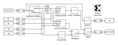
When using a uniform sampling scheme, the addresses and differences can be calculated by extracting, respectively, the most (MSB) and less (LSB) significant bits from the input x. But in our case, because the values stored inside the RAM blocks come from a nonuniform sampling scheme, we have to apply a more complex operation for calculating these values. This task is performed by the specific designed subsystem Difference_Address, as can be seen in the schematic top view (Figure 1) of the nonuniform LUT-based interpolator. Figure 1 shows the Difference_Address subsystem, two RAM blocks for storing the ordinate and the derivative, a block that multiplies the output of derivative RAM block with the difference , a block that adds this product with the output gotten from ordinate RAM block, and three delay blocks used to synchronize the data flow.
The subsystem Difference_Address can be seen in details in Figure 2. It has two outputs and two branches, one for calculating the addresses to be used by the RAM blocks and the other related to the calculation of the Differences . It is directly programmed by the parameters presented in Section 2 and illustrated in Tables 1 and 2. When we change the configuration parameters in accordance with the contents of the ordinate and derivative RAM blocks, we enable the LUT to interpolate different g(x) functions, according to different nonuniform sampling schemes. The Difference_Address subsystem is composed of nine blocks (six subsystems, two adders, and one binary point forcer), as it will be discussed in the following.
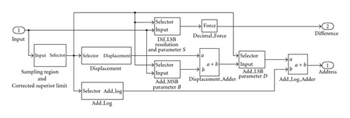
The first subsystem (Sampled Region and Corrected Superior Limit) in Figure 2 is configured by the Corrected Superior Limit (CSLn) parameters calculated by (3) and exemplified in column 3 of Table 2. It senses the input x, and outputs a selector signal that identifies the partition n where this input belongs. For instance, in the case of using the sampling scheme illustrated by Tables 1 and 2, for x = −0.97, it outputs a selector signal equal to 5, meaning that the input x belongs to the partition [x5, x6) = [−0.95904541015625, −0.98052978515625).
Based on the selector signal provided by subsystem Sampled Region and Corrected Superior Limit, the next two subsystems, Displacement and AddLog, output the values Dspn and Add log n calculated by (7) and (8). These both values are used to calculate the nonuniform RAM addresses via the two blocks named Displacement_Adder and Add_Log_Adder. Continuing on the example above, the provided selector signal equals to 5, implying Dspn = 1024 and Add logn = 78.
Keeping on the description of the Address branch of Figure 2, we have two subsystems that select a configurable number of bits from their inputs. The first one, named Add_MSB, slices a configurable number of the most significant bits of input x. This configurable number of selected bits is defined by the parameter Bn in (4). This output is added with the Displacement value Dspn, and a configurable number of its less significant bits, defined by the parameter Dn in (5), is selected by subsystem Add_LSB. Finally, the Address is calculated by adding this value with the parameter Add log n explained above and calculated by (8).
The output Difference is calculated by the configurable subsystem named Dif_LSB. It is configured by the parameters Sn in (6) and the sampling frequency fn in Table 1. This subsystem slices a configurable number (defined by parameter Sn) of the less significant bits of the input x and forces the binary point to a fixed position d = 14. An exception must be done on the sampling regions where fn = 215 because no interpolation is necessary: all possible values x of these regions are mapped one to one to a corresponding , and the differences are always made equal to zero.
The six subsystems discussed above are configured on the fly by the parameters enumerated in the example in Tables 1 and 2. These parameters are stored inside each subsystem by means of 28 memories (22 RAM blocks storing 2 positions each and 6 storing 22 positions). Their contents, as well as the contents of the 512 positions wide ordinate and derivative RAM blocks, can be changed on the fly, what enables this nonuniform LUT-based interpolator to represent different g(x) functions, according to different sampling schemes, as it will be seen in Section 4. The reconfiguration time is defined by the depth of the longest RAM block, the ordinate or derivative RAM blocks: the interpolator requires 512 clock cycles for a full reconfiguration.
The presented design was implemented using the softwares Integrated Software Environment (ISE) and System Generator (SysGen) from Xilinx, on a Spartan-3 development kit from Avnet with a XC3S2000-5 FG676 Spartan 3 FPGA. The synthesis details of this realization can be seen on Table 3.
| Property | Value |
|---|---|
| Device part type | XC3S2000 |
| Package type | FG 676 |
| Speed grade | −5 |
| Number of external IOBs | 304 out of 489 |
| Number of slices | 802 out of 30720 |
| Number of SLICEMs | 123 out of 10240 |
| Number of BUFGMUXs | 1 out of 8 |
| Number of RAMB16s | 32 out of 40 |
| Average connection delay | 2.281 ns |
| Maximum frequency | 151.717 MHz |
| Minimum period | 6.591 ns |
| Total power consumption | 636 mW |
| Junction temperature | 25°C |
4. Programmable Noise Generator
As a study case, the proposed nonuniform LUT-based interpolator was used as a programmable noise generator able to output noise with different Probability Density Functions (PDFs). A controlled level of approximation error is achieved by using the proposed programmable nonuniform sampling scheme.
The transformation function g1(x) has two poles located at the abscissas x = −1 and x = +1, which are characterized by high values of curvature and derivatives. Both the uniformly distributed input signal and the domain of g1(x) are represented by the interval [x1, xP+1) = [−1, +0.99993896484375). The ordinate of this function ideally goes from −∞ to +∞, what is expected since the output is an unlimited normally distributed signal.
One advantage of implementing a nonuniform sampling scheme for the interpolation of g1(x) is the lower RAM space necessary for storing both the ordinates and derivatives, allied to a lower approximation error. As a counterexample, if we use a uniform sampling scheme instead of the proposed nonuniform one, we would face high approximation error around the poles of (14), even using high frequency samplings, as seen in Figure 3. These graphs show the absolute approximation error verified when two different uniform sampling schemes were applied to the whole [x1, xP+1) domain: the upper graph shows the error for fn = 128, what requires the storage of in = 256 positions of ordinates plus in = 256 for derivatives; and the lower graph (observe the zoom on x axis) shows the error for the case where fn = 16384, that results in in = 32768 + 32768 = 65536 positions for both RAM blocks. The horizontal line in Figure 3 represents a boundary approximation error limit equal to 3.0518 × 10⁻⁵: the input values are 15 bits long, and any error lower than that boundary does not decrease the quality of the interpolation.
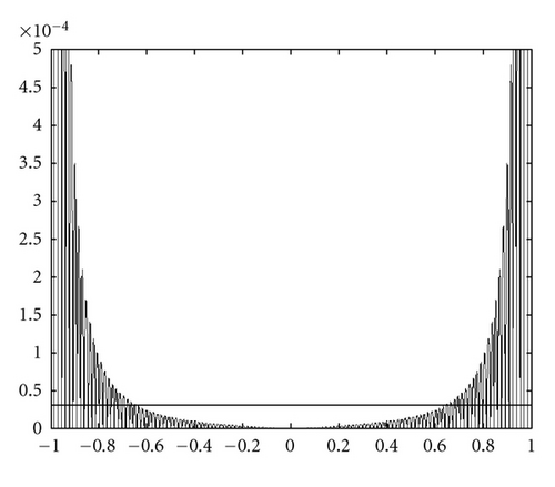
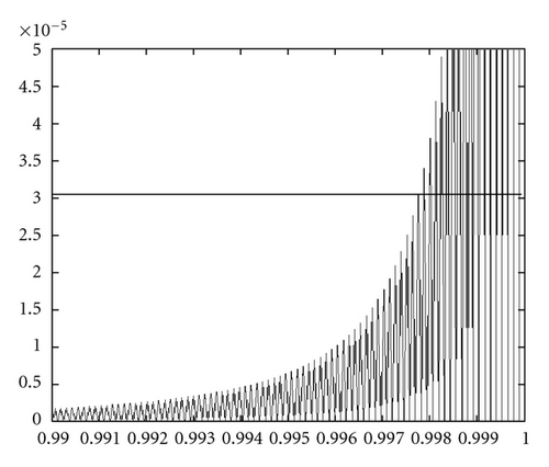
If a uniform sampling scheme is used, the only solution to keep the absolute approximation error below this boundary for all abscissas x would be to use fn = 32768, what makes the approximation error equal to zero for all possible abscissas x. This happens because, in this extreme case, there is not a really interpolation, but a one-to-one mapping of all possible input values x. But such linear sampling scheme requires a RAM block with a high depth equal to in = 65536 positions for storing , hard to implement on an FPGA due to the number of bits necessary to represent each stored value.
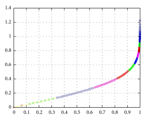
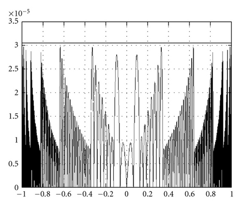
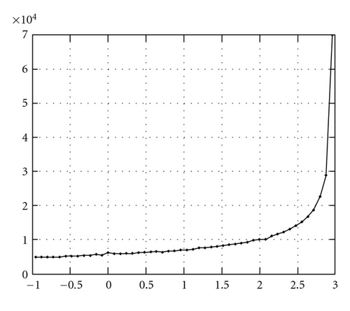
The solution is to use the proposed nonuniform sampling scheme which stores less ordinates and derivatives for input values around x = 0, and more samples near the poles x = +1 and x = −1, where the approximation error is bigger, saving significant amount of memory space (the proposed LUT-based interpolator reserves only 512 positions for each ordinate and derivative RAM blocks). This approach is graphically presented in Figure 4, where you can see the 1st quadrant of g1(x)—the 3rd quadrant is not displayed since it is symmetric in relation to the origin (0,0). The absolute approximation error obtained with this nonuniform approach remains under the boundary limit (3.0518 × 10⁻⁵) even near the poles of g1(x), as seen in Figure 5.
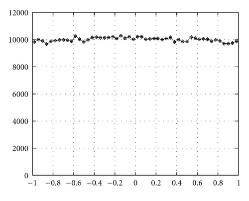
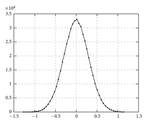
When the proposed programmable nonuniform LUT-based interpolator is configured to represent (14), according to the sampling scheme of Tables 1 and 2, it works as a Gaussian noise generator: by applying to its input a signal with a uniform PDF (Figure 6(a)), it outputs a signal with Gaussian PDF (Figure 6(b)).
Tables 1 and 2 are just one example of configuration data for the proposed programmable LUT-based interpolator. In this work, 3 different sampling schemes (α, β, and γ) were formulated. The sampling scheme α was the one demonstrated in Tables 1 and 2. The abscissas of sampling schemes α, β, and γ are plotted in Figure 7. As can be seen in these figures, there are sampling points on scheme α, on scheme β, and on scheme γ. As expected, the amount of sampling points is always smaller than the depth (equal to 512) of the two RAM blocks that store the corresponding ordinates and derivatives . Observe that the inclination on these graphs is inversely proportional to the sampling frequency fn of each partition n: the higher the frequency fn, the bigger the number of abscissas , and the smaller the inclination in Figure 7.
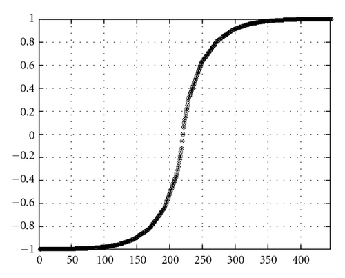
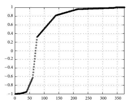
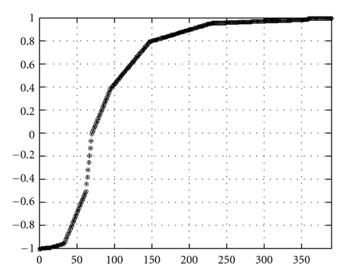
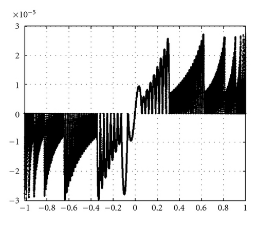
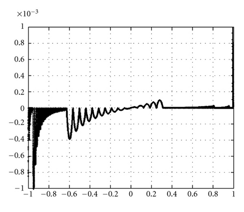
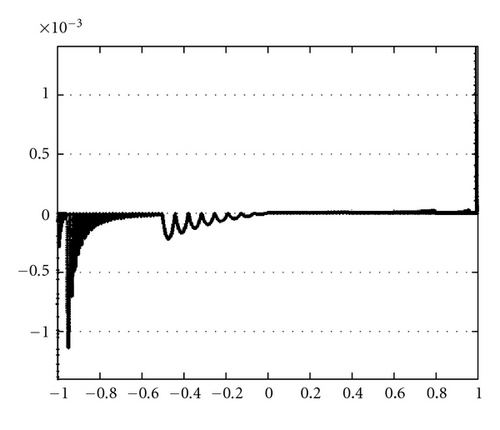
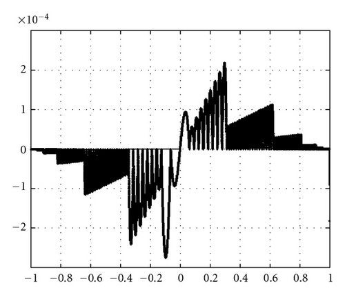
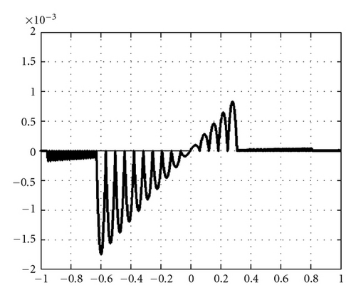
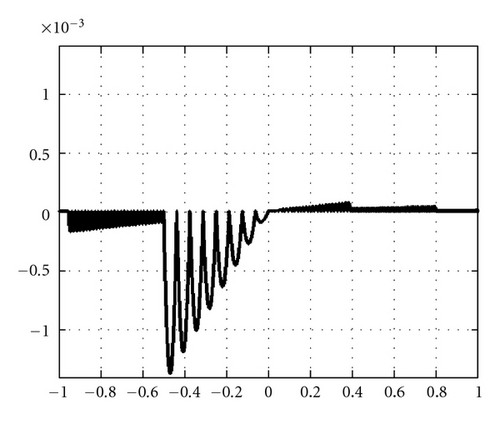
Each sampling scheme was designed to minimize the approximation error for x abscissa values belonging to the sampling region with higher fn values. As a matter of fact, high frequencies should be used for regions where g(x) presents a strong nonlinear behavior and low frequencies for regions with a linear behavior. For example, the sampling scheme α was specifically designed for the Gaussian transformation function (14). It applies high frequencies (fn = 16384) near the poles x = +1 and x = −1 and low frequencies (fn = 32) near the origin x = 0. The approximation error for the three sampling schemes α, β, and γ can be seen in Figure 8, in a case of using the displaced Gaussian transformation function (15), and in Figure 9, for the Cubic Function (18) case.
The frequency assignment of the P = 22 partitions for sampling schemes β and γ is presented in Table 4. The corresponding configuration parameters for these sampling schemes are calculated via (2) to (12) and are presented in Tables 5 and 6. Observe that the sampling limits xn for sampling scheme β are the same as sampling scheme α, only the frequencies fn are distributed differently. But in the sampling scheme γ, both sampling limits xn and the frequencies fn are distributed differently from sampling schemes α and β, what shows the flexibility for reconfiguring the designed programmable noise generator.
| n | xn [β] | fn [β] | xn [γ] | fn [γ] |
|---|---|---|---|---|
| 1 | −1,000000 | 4096 | −1,000000 | 1024 |
| 2 | −0,997700 | 4096 | −0,996000 | 1024 |
| 3 | −0,995400 | 4096 | −0,995400 | 4096 |
| 4 | −0,990300 | 1024 | −0,990000 | 1024 |
| 5 | −0,980500 | 1024 | −0,980500 | 1024 |
| 6 | −0,959000 | 128 | −0,959000 | 128 |
| 7 | −0,914100 | 128 | −0,914100 | 128 |
| 8 | −0,820400 | 128 | −0,700000 | 128 |
| 9 | −0,640700 | 32 | −0,500000 | 32 |
| 10 | −0,343800 | 32 | −0,343800 | 32 |
| 11 | −0,125100 | 32 | −0,125100 | 32 |
| 12 | 0,000000 | 32 | 0,000000 | 128 |
| 13 | 0,124900 | 32 | 0,200000 | 128 |
| 14 | 0,343600 | 256 | 0,400000 | 256 |
| 15 | 0,640500 | 256 | 0,700000 | 256 |
| 16 | 0,820200 | 1024 | 0,800000 | 1024 |
| 17 | 0,914000 | 1024 | 0,914000 | 1024 |
| 18 | 0,958900 | 8192 | 0,958900 | 8192 |
| 19 | 0,980400 | 8192 | 0,980400 | 8192 |
| 20 | 0,990100 | 512 | 0,990100 | 512 |
| 21 | 0,995300 | 512 | 0,995300 | 512 |
| 22 | 0,997600 | 16384 | 0,997600 | 16384 |
| — | 0,999938 | — | 0,999938 | — |
| n | PILn | CSLn | Bn | Dn | Sn | Dspn | Add logn | SPSn | MPSn | SPFn | MPFn |
|---|---|---|---|---|---|---|---|---|---|---|---|
| 1 | −1.00000000000 | −0.99761962890 | −11 | 12 | 3 | 2048 | 0 | −1.00000000000 | 1 | −0.99755859375 | 6 |
| 2 | −0.99755859375 | −0.99517822265 | −11 | 12 | 3 | 2048 | 0 | −0.99707037250 | 7 | −0.99511718750 | 11 |
| 3 | −0.99511718750 | −0.99029541015 | −11 | 12 | 3 | 2048 | 0 | −0.99462890625 | 12 | −0.99023437500 | 21 |
| 4 | −0.99023437500 | −0.98052978515 | −9 | 10 | 5 | 512 | 15 | −0.98828125000 | 22 | −0.98046875000 | 26 |
| 5 | −0.98046875000 | −0.95318603515 | −9 | 10 | 5 | 512 | 15 | −0.97851562500 | 27 | −0.95312500000 | 40 |
| 6 | −0.95312500000 | −0.90631103515 | −6 | 7 | 8 | 64 | 36 | −0.93750000000 | 41 | −0.90625000000 | 43 |
| 7 | −0.90625000000 | −0.81256103515 | −6 | 7 | 8 | 64 | 36 | −0.89062500000 | 44 | −0.81250000000 | 49 |
| 8 | −0.81250000000 | −0.62506103515 | −6 | 7 | 8 | 64 | 36 | −0.79687500000 | 50 | −0.62500000000 | 61 |
| 9 | −0.62500000000 | −0.31256103515 | −4 | 5 | 10 | 16 | 54 | −0.56250000000 | 62 | −0.31250000000 | 66 |
| 10 | −0.31250000000 | −0.12506103515 | −4 | 5 | 10 | 16 | 54 | −0.25000000000 | 67 | −0.12500000000 | 69 |
| 11 | −0.12500000000 | −0.00006103515 | −4 | 5 | 10 | 16 | 54 | −0.06250000000 | 70 | +0.00000000000 | 71 |
| 12 | +0.00000000000 | +0.06243896484 | −4 | 5 | 10 | 16 | 54 | +0.06250000000 | 72 | +0.06250000000 | 72 |
| 13 | +0.06250000000 | +0.31243896484 | −4 | 5 | 10 | 16 | 54 | +0.12500000000 | 73 | +0.31250000000 | 76 |
| 14 | +0.31250000000 | +0.63275146484 | −7 | 8 | 7 | 128 | −93 | +0.32031250000 | 77 | +0.63281250000 | 117 |
| 15 | +0.63281250000 | +0.81243896484 | −7 | 8 | 7 | 128 | −93 | +0.64062500000 | 118 | +0.81250000000 | 140 |
| 16 | +0.81250000000 | +0.91204833984 | −9 | 10 | 5 | 512 | −193 | +0.81445312500 | 141 | +0.91210937500 | 191 |
| 17 | +0.91210937500 | +0.95697021484 | −9 | 10 | 5 | 512 | −789 | +0.91406250000 | 192 | +0.95703125000 | 214 |
| 18 | +0.95703125000 | +0.98016357421 | −12 | 13 | 2 | 4096 | −789 | +0.95727539062 | 215 | +0.98022460937 | 309 |
| 19 | +0.98022460937 | +0.98822021484 | −12 | 13 | 2 | 4096 | −7803 | +0.98046875000 | 310 | +0.98828125000 | 342 |
| 20 | +0.98828125000 | +0.99212646484 | −8 | 9 | 6 | 256 | −168 | +0.99218750000 | 343 | +0.99218750000 | 343 |
| 21 | +0.99218750000 | +0.99603271484 | −8 | 9 | 6 | 256 | −168 | +0.99609375000 | 344 | +0.99609375000 | 344 |
| 22 | +0.99609375000 | +0.99981689453 | −13 | 14 | 1 | 8192 | −16009 | +0.99621582031 | 345 | +0.99975585937 | 374 |
| n | PILn | CSLn | Bn | Dn | Sn | Dspn | Add logn | SPSn | MPSn | SPFn | MPFn |
|---|---|---|---|---|---|---|---|---|---|---|---|
| 1 | −1.00000000000 | −0.99420166015 | −9 | 10 | 5 | 512 | 0 | −1.00000000000 | 1 | −0.99414062500 | 4 |
| 2 | −0.99414062500 | −0.99420166015 | −9 | 10 | 5 | 512 | 0 | −0.99218750000 | 5 | −0.99414062500 | 4 |
| 3 | −0.99414062500 | −0.98834228515 | −11 | 12 | 3 | 2048 | −9 | −0.99365234375 | 5 | −0.98828125000 | 16 |
| 4 | −0.98828125000 | −0.98052978515 | −9 | 10 | 5 | 512 | 9 | −0.98632812500 | 17 | −0.98046875000 | 20 |
| 5 | −0.98046875000 | −0.95318603515 | −9 | 10 | 5 | 512 | 9 | −0.97851562500 | 21 | −0.95312500000 | 34 |
| 6 | −0.95312500000 | −0.90631103515 | −6 | 7 | 8 | 64 | 30 | −0.93750000000 | 35 | −0.90625000000 | 37 |
| 7 | −0.90625000000 | −0.68756103515 | −6 | 7 | 8 | 64 | 30 | −0.89062500000 | 38 | −0.68750000000 | 51 |
| 8 | −0.68750000000 | −0.50006103515 | −6 | 7 | 8 | 64 | 30 | −0.67187500000 | 52 | −0.50000000000 | 63 |
| 9 | −0.50000000000 | −0.31256103515 | −4 | 5 | 10 | 16 | 54 | −0.43750000000 | 64 | −0.31250000000 | 66 |
| 10 | −0.31250000000 | −0.12506103515 | −4 | 5 | 10 | 16 | 54 | −0.25000000000 | 67 | −0.12500000000 | 69 |
| 11 | −0.12500000000 | −0.00006103515 | −4 | 5 | 10 | 16 | 54 | −0.06250000000 | 70 | +0.00000000000 | 71 |
| 12 | +0.00000000000 | +0.18743896484 | −6 | 7 | 8 | 64 | 6 | +0.01562500000 | 72 | +0.18750000000 | 83 |
| 13 | +0.18750000000 | +0.39056396484 | −6 | 7 | 8 | 64 | 6 | +0.20312500000 | 84 | +0.39062500000 | 96 |
| 14 | +0.39062500000 | +0.69525146484 | −7 | 8 | 7 | 128 | −83 | +0.39843750000 | 97 | +0.69531250000 | 135 |
| 15 | +0.69531250000 | +0.79681396484 | −7 | 8 | 7 | 128 | −83 | +0.70312500000 | 136 | +0.79687500000 | 148 |
| 16 | +0.79687500000 | +0.91204833984 | −9 | 10 | 5 | 512 | −773 | +0.79882812500 | 149 | +0.91210937500 | 207 |
| 17 | +0.91210937500 | +0.95697021484 | −9 | 10 | 5 | 512 | −773 | +0.91406250000 | 208 | +0.95703125000 | 230 |
| 18 | +0.95703125000 | +0.98016357421 | −12 | 13 | 2 | 4096 | −7787 | +0.95727539062 | 231 | +0.98022460937 | 325 |
| 19 | +0.98022460937 | +0.98822021484 | −12 | 13 | 2 | 4096 | −7787 | +0.98046875000 | 326 | +0.98828125000 | 358 |
| 20 | +0.98828125000 | +0.99212646484 | −8 | 9 | 6 | 256 | −152 | +0.99218750000 | 359 | +0.99218750000 | 359 |
| 21 | +0.99218750000 | +0.99603271484 | −8 | 9 | 6 | 256 | −152 | +0.99609375000 | 360 | +0.99609375000 | 360 |
| 22 | +0.99609375000 | +0.99981689453 | −13 | 14 | 1 | 8192 | −15993 | +0.99621582031 | 361 | +0.99975585937 | 390 |
As seen in Table 1, the scheme α distributes the P = 22 sampling frequencies fn symmetrically to the origin, with the lower frequencies near the origin, as can be graphically seen in Figures 8 and 9 (upper graphs): the semiarcs with bigger diameters (related to fn = 32) are located around the origin, in the interval −0.125 < x < 0.125. As seen in Table 4, the schemes β and γ distribute the lower sampling frequencies (fn = 32) on the intervals −0.64 < x < 0.34 and −0.5 < x < 0.0, respectively, as can be graphically seen in Figures 8 and 9((b) and (c) graphs, resp.).
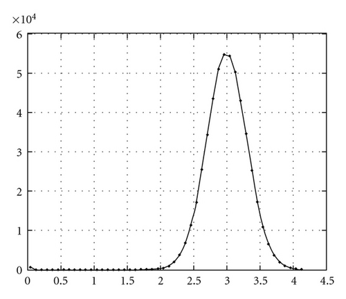
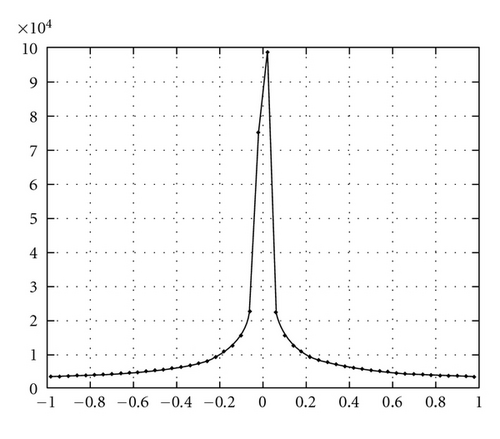
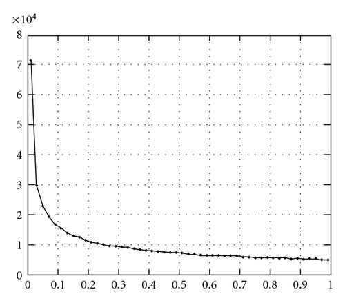
The designed programmable noise generator can generate different noise signals by properly filling the ordinate and the derivative RAM blocks (Figure 1) and configuring its internal parameters on the Difference_Address subsystem (Figure 2). For example, Figure 10 shows the Probability Density Functions (PDFs) of four different signals produced by the programmable noise generator when: (1) its input is fed with a uniform distributed noise, (2) it is configured with the sampling scheme α, and (3) it was configured to interpolate four different functions: the Displaced Error Function (15), the Cubic Function (18), the first (19), and the second (20) Quadratic Function.
5. Conclusion
A programmable Look-Up Table-based interpolator with nonuniform sampling scheme was implemented using a Avnet development kit containing an XC3S2000-5 FG676 Xilinx Spartan-3 FPGA. This LUT-based interpolator can be programmed on the fly by loading the proper configuration parameters presented in Section 2, including the ordinate and derivative, inside RAM blocks. The complete reconfiguration takes 512 clocks cycles. When these parameters are changed, they can interpolate different g(x) functions, sampled according to different nonuniform sampling schemes. The ability of changing the sampling scheme allows the minimization of both the approximation error and memory space: for instance, the sampling schema α (Table 1) applied to (14) was able to keep the approximation error below a threshold of 3.0518 × 10⁻⁵ while reducing the memory usage to 2.71% for a Gaussian noise generator application.
As a study case, the LUT-based interpolator was used as the core of a programmable noise generator able to output signals with different Probability Density Functions (PDFs). The flexibility of this design was proved by interpolating 8 different g(x) functions, according to 3 different nonuniform sampling schemes (α, β, and γ) described in Tables 1 and 4, each one defining P = 22 partitions each characterized by a chosen sampling frequency fn.
As future work, we recommend the implementation of a programmable nonuniform LUT-based interpolator with a domain not fixed to [x1, xP+1) = [−1, +1) and where the number P of sampling regions can be changed on the fly.


