Assessment of different interpolation algorithms for daily rainfall spatial distribution in the Var catchment, France
Abstract
To have effective water resource management, the distributed hydrological models are commonly applied for supporting the decision-making processes. Among different inputs, the spatial distributed rainfall plays significant role in those model simulations. Many interpolation methods have been developed for generating distributed rainfall based on measurement samples. However, depending on the catchment characteristics and data availability, the suitable interpolation algorithm is case-dependent. This paper presents one operational approach for determining the resonable interpolation algorithm in a complex large catchment (Var catchment, France). Based on the daily rainfall data (2008–2014) collected from 16 stations in the Var catchment, six different interpolation approaches including: inverse distance weight (IDW), spline, kriging with linear and spherical semi-variogram models and geographically weighted regression considering elevation effects and the combined impacts of elevation and distance to the sea were tested. Integrated the results of statistical and modeling assessments, the 400 m resolution distributed rainfall generated by IDW algorithm shows high preference in generating distributed rainfall in the Var catchment. Moreover, the strategy described in the article also shows promising acceptability for other catchments.
1 INTRODUCTION
Challenged by effects of global trends such as the climate change and the growing urbanization, management of water resources is getting more and more complicated. To efficiently harmonize various social demands, the distributed hydrological models are commonly applied for supporting the water-related decision-making process (Gourbesville et al., 2018). The distributed rainfall, as one of the major model inputs, has significant impact on the simulation performance (Bárdossy & Das, 2008; Beven, 2011; Chen et al., 2017; Fraga et al., 2018; Huard & Mailhot, 2006; Kim et al., 2018; Ly et al., 2011; Singh, 1998; Vo & Gourbesville, 2014). To have precise representation of the rainfall condition in a study catchment, many interpolation approaches have been developed for converting the rainfall samples to distributed rainfall intensity maps. Numerous research have been carried out for determining the most suitable algorithm for generating distributed rainfall in different catchments (Basistha et al., 2008; Buytaert et al., 2006; Dirks et al., 1998; Hutchinson, 1995; Nalder & Wein, 1998; Newlands et al., 2010; Oke et al., 2009; Price et al., 2000; Tao et al., 2009; Vicente Serrano et al., 2003; Vo & Gourbesville, 2014). The previous achievements could be summarized: (1) the main differences among various interpolation algorithms are their conceptual formulations and mathematical constructions (Burrough & McDonnell, 1998); (2) the best rainfall interpolation approach is intrinsically case-dependent (Bennett et al., 2013); (3) comparing to some “complex” interpolation approaches, which take into account many factors, the “simple” method is desirable to be firstly implemented at the targeted area unless it has been proved to be inadequate (Robson, 2014); (4) to comprehensively evaluate interpolation performance, applying the cross validation method could be an operational approach (Mair & Fares, 2011; Nalder & Wein, 1998; Vo & Gourbesville, 2014); and (5) due to the higher randomness of short term rainfall event, most of the previous studies were focused on the long term interpolation (monthly or annual rainfall) (Boer et al., 2001; Carrera-Hernández & Gaskin, 2007; Goovaerts, 2000; Hevesi et al., 1992), the acceptability of the validated method for estimating short term event (daily or hourly rainfall) is necessary to be further assessed.
The Var catchment (2800 km2) is the largest river basin in the French Mediterranean region characterized by the conspicuous elevation variation from the sea level up to over 3000 m (Figure 1). Since 19th century, human activities have significantly increased in this area and modified the regional terrain, especially at the lower Var Valley, where the fifth biggest city of France (NICE) is located at the outlet of the catchment. The catchment rainfall is generally affected by the Mediterranean climate with wet winter and dry summer. The difference between the total amounts of the different seasonal rainfall could reach more than 80%.
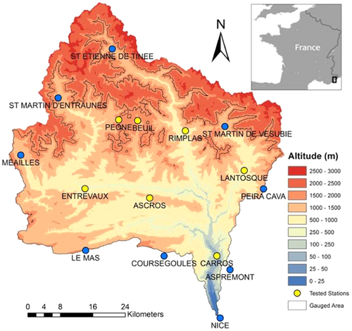
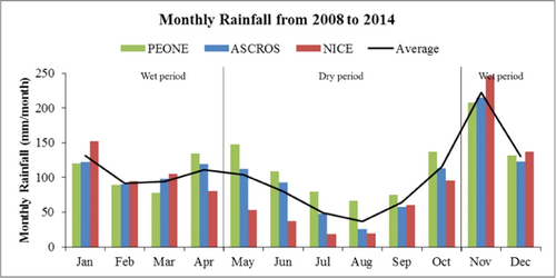
To define the best interpolation algorithm for generating distributed rainfall in Var catchment, the daily rainfall time series recorded at 16 stations in period 2008–2014 has been collected. The stations' elevations vary from 2 m (NICE) up to 1784 m (PEONE), covered 75% of the catchment area. Extracts and plots the monthly rainfall of three different stations located at upper (PEONE), middle (ASCROS) and lower (NICE) parts of the catchment, the joint effects of geological elements (e.g., elevation variation) and regional factors (e.g., characteristics of Mediterranean climate) show high impacts on the Var rainfall distribution (Figure 2). Obviously, the Mediterranean climate behaviors have strong influences on the temporal rainfall distribution that both wet and dry period in this catchment strongly affected by the Mediterranean climate. But for the spatial distribution of rainfall in the Var catchment, the elevation variation also plays significant role. In the Mediterranean winter, most of the extreme rainfall is landed at the seas side area, and with the increasing of the surface elevation, the total amount of monthly rainfall shows a decreasing trend. However, in the spring season, when the impact of regional climate is decreasing, the local topographic factors start to have more obvious impacts on the rainfall spatial distribution. The monthly rainfall amount is increasing with the rise of surface elevation.
2 METHODS AND MATERIALS
Obviously, the main difference among various interpolation algorithms lies on the estimation of contribution weight of the each sample point. The interpolation methods can be classified into two categories: deterministic methods and geostatistical methods. The deterministic methods deem the contribution weight of each sample point in relation with its distance to the estimated point. Many algorithms have been created based on this hypothesis such as Thiessen polygon method, spline method (SPL) and inverse distance weight (IDW) method. Those deterministic methods are considered as simpler approaches and commonly applied in the relatively flat zones (Ly et al., 2013). However, for the catchment having more complex topography, due to the relation between rainfall and surface elevation (Allamano et al., 2009; Basist et al., 1994; Brunsdon et al., 2001; Chow et al., 1988; Gouvas et al., 2009; Groisman & Legates, 1994; Johansson & Chen, 2003; Johnson & Hanson, 1995; Sevruk, 1997; Sinclair et al., 1997), the deterministic method is often replaced by the geostatistical method, which constitutes a discipline connecting mathematics and earth sciences (Ly et al., 2013). The core technique applied in the geostatistical interpolation approach is to characterize the spatial dependences between estimations and observations through certain semi-variogram models. However, due to the negative weights appears when the estimated points closer to the outlying border, the geostatistical method could produce negative estimations in the rainfall distribution (Deutsch, 1996).
In practice, to define the best interpolation algorithm for generating the rainfall spatial distribution at the targeted catchment, the performances of both deterministic and geostatistical methods need to be assessed and evaluated through a comprehensive comparison. Among different assessment approaches, the cross validation method has been proved as one of effective tools for reaching such objective (Mair & Fares, 2011; Nalder & Wein, 1998; Vo & Gourbesville, 2014). By temporarily removing one sampled point from the database and re-estimating the removed values based on the remaining data through different interpolation methods, the cross validation approach allows the users to apply many statistic indexes to have a systemic evaluation of the performances of all tested algorithms in many aspects.
In this study, six interpolation algorithms has been assessed including: IDW method, SPL, ordinary kriging method with linear and spherical semi-variogram models (OKL and OKS), and geographically weighted regression method respectively taken into account the impact of elevation and the combined influence of elevation and distance to the sea (GWRZ and GWRZD).
The kriging interpolation method is well known as one of the best solutions of interpolation, which consisted of a family of least-square linear regression algorithms applied for estimating random fields from observed data (Goovaerts, 1997, 1998). The equations in kriging method are similar as IDW method, but the weight coefficient here is not only referenced by the distance between the gauged points and the predication locations but also calculated with overall spatial arrangement of the measured points. To apply the spatial arrangement in the weights estimation, the spatial autocorrelation should be quantified. In this assessment, the spherical and linear kriging interpolation process were implemented in the function available in ArcGIS software. And the GWR interpolation method is a new local spatial statistical method used to examine and determine the spatial non stationary distribution when the relationships among variables vary from location to location (Fotheringham et al., 2003). In this research, by using the ArcGIS software, the GWR function taking into account the elevation difference was implemented in the assessment.
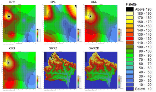
In the statistical assessment, the cross validation method has been applied for evaluating the performances of those interpolations. In addition, a distributed hydrological model has been also implemented in this research to find the best rainfall interpolation approach in the Var catchment (Figure 3).
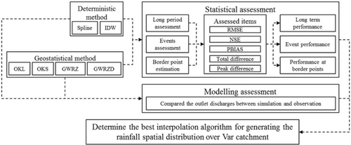
Depending on the sample distribution, the interpolation area can be generally split into two parts: “inside” part, where surrounded by measured samples, and the “border” part, where outside the gauged area but inside the interpolation domain. In the statistical assessment, the cross validation approach is first implemented on the “inside” part for evaluating the different interpolations' performances for both long term period (2008–2014) and short term events (floods and drought) with the interpolation special resolution of 100 m and temporal resolution in daily step. After, two points located at the domain borders (MEAILLES and PEONE) are selected for the analysis of estimating accuracy of different interpolation: one is the MEAILLES located at the west border of the Var monitoring network, and the other one is highest gauging station (PEONE, 1784 m) in this area, which can be considered as the elevation border.
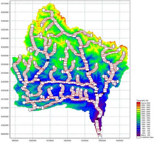
Beside the statistical assessment, in this research, one existing MIKE SHE model (Ma et al., 2020) in the Var catchment is applied for implementing the modeling assessment of different rainfall interpolations (Figure 4). As a deterministic distributed hydrological model, the MIKE SHE simulation was set up within 100 m resolution of overland flow and coupled with MIKE 11 model consisted with 52 branches described by 1238 cross sections. The rainfall distribution generated by various interpolation methods are considered as the only changing variable for launching the simulations. And simulations' performances are evaluated by comparing the outlet runoff from calculations and observation.
3 RESULTS AND DISCUSSION
3.1 Statistical assessment
Implementing the cross validation approach on the seven tested sample points (Figure 1), the statistical performances of six different rainfall interpolations in the Var catchment are showed in Table 1. Compared to the observed values, the interpolated daily rainfall in period 2008–2014 are 7%–10% over-estimated. The average difference of total amounts of rainfall between each simulation and observation is in range between 592.80 and 790.81 mm. The IDW and GWRZ methods, which have lower RMES (3.24 and 3.28) and higher NSE (0.86), show better performances than the rest of approaches for generating daily rainfall distribution in the Var catchment.
| Approaches | RMSE (mm/day) | NSE (−) | PBIAS (%) | ∆Total rainfall (mm) |
|---|---|---|---|---|
| IDW | 3.24 | 0.86 | 8.19 | 630.51 |
| SPL | 4.13 | 0.77 | 8.99 | 691.87 |
| OKS | 3.41 | 0.84 | 10.15 | 781.18 |
| OKL | 3.41 | 0.84 | 10.36 | 797.19 |
| GWRZ | 3.28 | 0.86 | 7.70 | 592.80 |
| GWRZD | 3.79 | 0.81 | 10.27 | 790.81 |
- Abbreviations: IDW, inverse distance weight; NSE, Nash-Sutcliffe coefficient; PBIAS, percentage bias; RMSE, root mean squared error; SPL, spline method.
This long period assessment is more focusing on assessing the ability of the simulated rainfall in representing the general rainfall condition (2008–2014) in the Var catchment. For having a comprehensive view of the various tested interpolations, the detailed analysis of the short term events (e.g., floods and drought) is necessarily needed.
Three hydrological events are selected for short term assessing in the Var catchment (Table 2) which defined by the local municipality (Zavattero et al., 2016). Consdiering the topography variation of the Var catchment which led the time lag of its flood propagation less than 12 h, the assessment of this study is set up in daily time step. For both two floods (in the spring and winter), the total estimated rainfall generated by all six interpolations is higher than the observation. Moreover, except the SPL rainfall, all other interpolation peak rainfall is higher than the observed value. Among six tested interpolations, the rainfall generated by IDW method shows the best performance in both two floods (spring flood: April 20, 2013–May 09,2013; winter flood: January 11, 2011–November 11, 2011) with higher NSE values (0.97 and 0.98) and lower peak rainfall differences (0.85 and 5.28 mm/day). For the drought event (July 20, 2012–August 08, 2012), although the NSE value of IDW rainfall is obviously reduced (0.73) and the interpolated total amount of rainfall is slightly under-estimated (−1.39 mm), compares to other interpolations, the IDW still shows relatively higher performance.
| Events | Assessment factors | IDW | SPL | OKS | OKL | GWRZ | GWRZD |
|---|---|---|---|---|---|---|---|
| Spring flood (20 days) | RMSE (mm/day) | 2.00 | 2.30 | 2.14 | 2.19 | 2.25 | 1.84 |
| NSE (−) | 0.97 | 0.96 | 0.96 | 0.96 | 0.95 | 0.97 | |
| PBIAS (%) | 2.64 | 0.58 | 3.63 | 4.56 | 3.18 | 3.56 | |
| ∆Total rainfall (mm) | 2.02 | 0.29 | 2.72 | 3.72 | 5.23 | 3.52 | |
| ∆Peak rainfall (mm/day) | 0.85 | −1.77 | 0.92 | 0.95 | 3.79 | 3.09 | |
| Winter flood (11 days) | RMSE (mm/day) | 4.49 | 7.56 | 5.87 | 6.00 | 6.27 | 7.99 |
| NSE (−) | 0.98 | 0.95 | 0.97 | 0.96 | 0.97 | 0.94 | |
| PBIAS (%) | 5.65 | 3.90 | 9.00 | 7.73 | 10.82 | 7.29 | |
| ∆Total rainfall (mm) | 9.92 | 5.64 | 16.86 | 13.85 | 23.11 | 10.01 | |
| ∆Peak rainfall (mm/day) | 5.38 | 5.78 | 5.11 | 2.66 | 7.02 | 3.52 | |
| Drought (19 days) | RMSE (mm/day) | 1.59 | 1.97 | 1.83 | 1.80 | 1.46 | 1.56 |
| NSE (−) | 0.73 | 0.59 | 0.64 | 0.65 | 0.74 | 0.72 | |
| PBIAS (%) | −12.19 | 5.48 | −1.91 | −2.63 | 2.46 | −0.66 | |
| ∆Total rainfall (mm) | −1.39 | 0.66 | −0.47 | −0.38 | 1.13 | −0.04 |
- Note: N.S. Spring flood: April 20, 2013–May 09,2013; Winter flood: January 11, 2011–November 11, 2011; Drought: July 20, 2012–August 08, 2012.
- Abbreviations: IDW, inverse distance weight; NSE, Nash-Sutcliffe coefficient; PBIAS, percentage bias; RMSE, root mean squared error; SPL, spline method.
In the assessment of “border” estimation, at both two different “border” stations, the IDW rainfall shows the best performance with highest NSE values (0.90 and 0.78) and lowest RMSE (2.77 and 4.00 mm/day) (Table 3). At the elevation border (PEONE), compares to the observation, the total amount of IDW rainfall (2008–2014) is −285.21 mm under-estimated. And at the west border (MEAILLES), where less sample references nearby, the total amount of IDW rainfall is over-estimated with 277.73 mm. Moreover, for the peak rainfall in both spring and winter floods, due to the neglecting of elevation impacts, the IDW rainfall at the places above the maximum gauging elevation (1784 m) is slightly over-estimated in the spring flood (0.76 mm/day), but under-estimated during the winter extreme rainfall event (−8.11 mm/day).
| Assessment factors | IDW | SPL | OKS | OKL | GWRZ | GWRZD |
|---|---|---|---|---|---|---|
| PEONE (1784 m) | ||||||
| RMSE (mm/day) | 2.77 | 3.32 | 2.80 | 2.80 | 3.10 | 3.12 |
| NSE (−) | 0.90 | 0.86 | 0.90 | 0.90 | 0.88 | 0.88 |
| PBIAS (%) | 3.46 | −1.90 | 0.34 | 0.88 | −9.07 | −9.48 |
| ∆Total rainfall (mm) | −285.21 | 156.83 | −28.11 | −72.50 | 747.97 | 782.26 |
| ∆Total drought rainfall (mm) | −0.57 | 5.37 | 3.55 | 2.78 | 7.38 | 7.58 |
| ∆Spring peak rainfall (mm/day) | 0.76 | 7.51 | 3.34 | 3.29 | 7.70 | 7.26 |
| ∆Winter peak rainfall (mm/day) | −8.11 | 21.29 | 6.77 | 6.13 | 12.29 | 11.38 |
| MEAILLES (1090 m) | ||||||
| RMSE (mm/day) | 4.00 | 7.64 | 4.41 | 4.30 | 4.24 | 7.16 |
| NSE (−) | 0.78 | 0.19 | 0.73 | 0.74 | 0.75 | 0.29 |
| PBIAS (%) | −3.42 | −33.35 | −12.74 | −11.35 | 0.05 | 0.82 |
| ∆Total rainfall (mm) | 277.73 | 2704.88 | 1033.44 | 920.65 | −3.76 | −66.33 |
| ∆Total drought rainfall (mm) | 1.88 | 39.95 | 9.21 | 8.84 | −1.77 | −4.41 |
| ∆Spring peak rainfall (mm/day) | −3.74 | 27.62 | 7.65 | 6.44 | −9.15 | −9.63 |
| ∆Winter peak rainfall (mm/day) | 8.39 | 125.18 | 56.29 | 51.56 | −13.47 | −22.39 |
- Abbreviations: IDW, inverse distance weight; NSE, Nash-Sutcliffe coefficient; PBIAS, percentage bias; RMSE, root mean squared error; SPL, spline method.
Comprehensively considered the statistical performances of all six tested daily rainfall interpolations, the IDW approach shows highest performance in the Var catchment. This result is also confirmed by the research of Tao et al. (2009), who claimed the IDW approach is suitable for generating spatial distributed rainfall in small catchment in Lyon, France.
3.2 Modeling assessment
In parallel, all the spatial distributed rainfall generated by six tested interpolations within same spatial resolution (400 m) (Figure 5) were used as inputs in an existing MIKE SHE model to have modeling assessment. All simulations are set-up with daily time step from 2008 to 2014. Compares to the observed discharges at the outlet of the catchment (NICE), the simulated runoff with IDW interpolated rainfall has lowest difference of total amount of runoff (3284.12 m3) and higher NSE value (0.51) (Table 4). The IDW peak flows in spring (April 30, 2013) and winter (November 04, 2011) are both under-estimated with 7.16% and 8.1%, respectively, its lowest discharge during the drought period (August 19, 2012) is slightly over-estimated (0.76 m3/s). Although the GWRZ and GWRZD methods shows higher preference in simulating the peak flow in spring and winter, considering the total water amount generated by those two interlopation approaches are much higher then the observation (8746.89 and 10206.74 m3), the IDW method is determined as the most reasonable interpolation method for generating the special distributed rainfall in the Var catchment. One of the main reason of GWRZ and GWRZD to over-estimated the total water amount could be due to the lower resolution of DEM data applied in this study which can not be well-represented the reality. Moreover, the method of GWRZ and GWRZD which linearly considered the impacts of elevation variation but not can consider the mountain effects which let the rainfall to accumulate and to land only at a certain part of the catchment, with less gauging stations distributed at higher elevation area, the interpolation methods which considered the attitude impacts may not produce better results due to the data limitation.
| Assessment factors | IDW | SPL | OKS | OKL | GWRZ | GWRZD |
|---|---|---|---|---|---|---|
| RMSE (m3/s) | 38.18 | 35.61 | 38.29 | 38.34 | 39.99 | 39.49 |
| NSE (−) | 0.51 | 0.57 | 0.51 | 0.50 | 0.46 | 0.47 |
| PBIAS (%) | 2.21 | 6.46 | 3.38 | 3.73 | 5.89 | 6.87 |
| Winter flood Q (m3/s) | 844.80 | 907.56 | 873.77 | 887.57 | 921.81 | 929.04 |
| Winter flood ∆Q (m3/s) | −65.20 | −2.44 | −36.23 | −22.43 | 11.81 | 19.04 |
| Spring flood Q (m3/s) | 471.42 | 496.67 | 481.69 | 483.15 | 503.92 | 523.24 |
| Spring flood ∆Q (m3/s) | −41.58 | −16.33 | −31.31 | −29.85 | −9.08 | 10.24 |
| Drought Q (m3/s) | 15.06 | 16.58 | 15.27 | 15.09 | 16.05 | 15.56 |
| Drought ∆Q (m3/s) | 0.76 | 2.28 | 0.97 | 0.79 | 1.75 | 1.26 |
| Total Q (m3) | 151794.75 | 158102.39 | 153524.99 | 154054.03 | 157257.52 | 158717.37 |
| Total ∆Q (m3) | 3284.12 | 9591.76 | 5014.36 | 5543.40 | 8746.89 | 10206.74 |
- Note: N.S. Spring flood: April 20, 2013–May 09, 2013; Winter flood: November 01, 2011–November 11, 2011; Drought: July 20, 2012–August 08, 2012.
- Abbreviations: IDW, inverse distance weight; NSE, Nash-Sutcliffe coefficient; PBIAS, percentage bias; RMSE, root mean squared error; SPL, spline method.
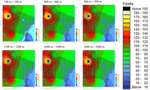
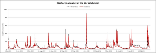
In the distributed hydrological model simulation, the resolution of the inputted rainfall distribution could also have impacts on the simulation performance. Thus, the IDW distributed rainfalls within six different resolutions (Figure 6) were used as inputs in the MIKE SHE model for determining the most suitable rainfall spatial resolution in the Var catchment. Taking the example of the winter flood at 2011, by decreasing the rainfall spatial resolution from 2000 to 100 m, no evident difference of total rainfall and simulated outlet runoff among six simulations have been observed. Therefore, considering the size of the input file, the 400 m resolution (33,345 cells) is defined as the suitable resolution of the spatial distributed rainfall in this catchment. The MIKE SHE simulated outlet hydrograph is showed in Figure 7, which well represents the trend and fluctuation of the river discharge in period 2008–2014.
4 CONCLUSION
The spatial distributed rainfall is one of most significant input variable of the simulation. This article presents one effective approach for determining the best rainfall interpolation method in a complex large catchment (Var catchment 2800 km2). Six different interpolation algorithms have been analyzed through statistical and modeling assessments. Individually evaluating the interpolation performance of longer period (2008–2014), short term (floods and drought) and the accuracy of “border” estimation, the IDW interpolation method has been defined as the most reasonable interpolation approach for generating spatial distributed daily rainfall based on 16 gauging stations in the Var catchment. In parallel, with the existing deterministic distributed hydrological model (MIKE SHE) in the Var catchment, all six interpolated rainfalls have been tested by the modeling assessment. Respectively, compares the outlet discharges of six simulations to the observation, with high NSE value, less RMES and difference of total amount of discharge and peak discharge, the IDW algorithm has been confirmed as the best interpolation approach in the Var catchment. In addition, similar conclusion could be also found in the research of Tao et al. (2009) in small catchment in Lyon. After the suitable interpolation method being identified, the resolution impacts of rainfall distribution on the hydrological simulation are further assessed in this research. Considering the similarity of total rainfall with different resolutions and the size of the input file, the 400 m resolution distributed rainfall generated by IDW interpolation has been finally determined as the best interpolation approach for producing daily rainfall in the hydrological modeling simulation in the Var catchment. The strategy applied in this research shows higher acceptability to use for identifying the suitable rainfall interpolation approach in other catchments with different data availabilities.
ACKNOWLEDGMENTS
This research is currently developed within the AquaVar project with the support of Metropole Nice Côte d'Azur, Agence de l'Eau Rhône Mediterranée, University of Nice Sophia-Antipolis, Conseil Départemental des Alpes-Maritimes and Meteo France. The work benefited from the data provided by the Metropole Nice Côte d'Azur, Conseil Départemental des Alpes-Maritimes, Meteo France, and H2EA. Part of this research is funded by the National Key R&D Program of China (2023YFC3006702).
ETHICS STATEMENT
None declared.
Open Research
DATA AVAILABILITY STATEMENT
Author elects to not share data.


