The applicability of automated marine clay gully delineation using deep learning in Norway
Alexandra Jarna Ganerød and Mikis van Boeckel contributed equally to this work.
Abstract
Gullies and ravines are common landforms in raised marine fine-grained deposits in Norway. Gullies in marine clay are significant landforms indicative of soil erosion and natural hazards and are of high conservation value. As a result of the substantial impact of human intervention over the past century, marine clay gullies are now red-listed. To monitor the condition of these landforms, we need to improve our understanding of their spatial extent, complexity and morphology. We explore the applicability of automated approaches that use a methodology of combining deep learning (DL), fully convolutional neural networks (FCNNs) and an unmodified U-Net model with ArcPy libraries and ground truth data to derive a high-resolution map of gullies in raised marine fine-grained deposits. Predictors used comprise solely terrain derivatives to broaden the usage of the pre-trained model to other regions. Our best model achieved a precision score of 0.82 and a recall of 0.75. We find that our pre-trained model can successfully predict gullies, also in blind-test areas. The model performs better in regions with similar geological settings, scoring a length-weighted overlap of >70% with reference datasets. The novelty of this study is that we demonstrate that the model's applicability for mapping routines increases when we post-process the predictions by eliminating noise, especially by using the predictions derived from ensembled models. We, therefore, conclude that the pre-trained models can effectively be used to supplement the geomorphological mapping of marine clay gullies in Norway. The outcome of this research contributes towards mapping the spatial extent and condition of red-listed landforms in Norway, as well as the development of monitoring systems for future landscape change.
1 INTRODUCTION
During and after the rapid deglaciation of the Scandinavian ice sheet, the retreating outlet glaciers fed fjords and sea inlets with large quantities of fine-grained glaciomarine and marine sediments. As a result of the ongoing post-glacial isostatic rebound after deglaciation, these marine deposits, commonly consisting of clay stratified with silt and sand, gradually emerged above sea level (Hansen et al., 2007; Reite, Sveian, & Erichsen, 1999). During regression, these emerging flats of marine deposits tend to develop into a characteristic landscape called marine clay landscapes (Erikstad, 1992) or gully landscapes (Bergqvist, 1990; Hamre et al., 2021). The gully landscapes in Norway have a rough topography mainly controlled by gully erosion, incision by rivers and landsliding in quick clay.
Characteristics of marine clay landscapes are gullies and ravines. These narrow, often v- or u-shaped landforms have steep sides and head scarps incised into unconsolidated material (Higgins & Coates, 1990). Erosion along these gullies involves the removal of sediment because of concentrated flow converging towards lower points of the watershed and is often associated with groundwater seepage and shallow sliding (Bridge, 2003). With the narrow channels' increasing size, depth and branching, gullies gradually transit into ravines. Gullies and ravines may have permanent or intermittent flowing streams that control the local drainage network and influence the direction of groundwater flow. For simplicity, in this paper, we do not differentiate between gully and ravine and use the term marine clay gully to describe the narrow channel incised into fine-grained glaciomarine and marine deposits.
Gullies in marine fine-grained deposits are of high conservation value due to the marine clay's high nutrient content and moisture-holding capacity (Erikstad, 1992; Hamre et al., 2021). Networks of the gully systems are essential wildlife corridors (Blindheim & Abel, 2002) and facilitate a large diversity of habitat types (Blindheim et al., 2018; Jansson & Høitomt, 2013). Agricultural policies of levelling and ploughing, along with urban development, caused the gully landscape to be subjected to substantial landscape change over the past century (Erikstad, 1992; Hamre et al., 2021), which resulted in the red-listing of the landform marine clay gully (Erikstad et al., 2018).
As part of developing a nationwide conservation plan for preserving the gully landscape, there is a need to map and monitor the change and condition of marine clay gullies. Moreover, because many quick-clay landslides are initiated in marine clay gullies, an overview of the spatial extent and development of these landforms contributes to improving hazard assessment. The establishment of monitoring systems with repeated mapping and comparison of time series, areas of comprehensive vertical erosion and migration of gullies may attract attention to hazard mitigation (Ryan et al., 2022) and soil erosion (Barneveld, Stolte, & van der Zee, 2022; Kværnø & Krzeminska, 2021).
Earlier studies on the delineation and condition of marine clay gullies in Norway have relied on manual mapping of aerial images (Hamre et al., 2021) or high-resolution terrain models and surficial geological maps (Christoffersen et al., 2021; van Boeckel et al., 2022; van Boeckel et al., 2023). Approaches to automated delineations of gullies outside of Norway have also developed rapidly but have mostly focused on gully erosion susceptibility and comparison of different machine-learning algorithms (Arabameri et al., 2020; Arabameri et al., 2022; Band et al., 2020; Chen et al., 2021; Chuma et al., 2023; Gayen et al., 2019; Mohebzadeh et al., 2022; Setargie et al., 2023). Setargie et al. (2023) used a Random Forest-based approach in Ethiopia, combining 164 manually mapped gullies with 20 predictors. The predictors used in this study included elevation, slope, Topographic Positioning Index (TPI), Terrain Roughness (TR), profile curvature, convergence index, soil type and distance from streams. Band et al. (2020) applied a deep learning approach using 132 gully erosion locations with 13 independent variables, comprising lithology, rainfall, Stream Power Index (SPI), and Topographic Wetness Index (TWI) and terrain derivatives, similar to the study from Setargie et al. (2023). Liu et al. (2022) also tested the applicability of automated approaches in new blind-test areas by applying U-net for image segmentation using satellite (QuickBird-2, Pleiades: worldView-03) with obtained UAV image data (worldView2 and PHANTOM 4 RTK). Here, the authors successfully used vector lines of gullies as ground truth data but provided limited information on the accuracy of delineation of the depressions. On the other hand, Arabameri et al. (2021) and Roy and Saha (2022) applied ensemble models with conventional machine learning algorithms. Lately, U-net and deep learning have been applied in different variations to map gully erosion (Aouragh et al., 2023; Chen et al., 2023; Gholami et al., 2023; Malik et al., 2021). They used topographical and hydrological gully erosion conditioning factors such as rainfall, distance from the river, surface runoff, length of overland flow and topographical wetness index. Although the studies mentioned above succeeded in identifying and delineating the gullies, little is known about automatic differentiations of gullies impacted by human interventions, such as agricultural levelling, and how these predictions can further be used for geomorphological mapping routines.
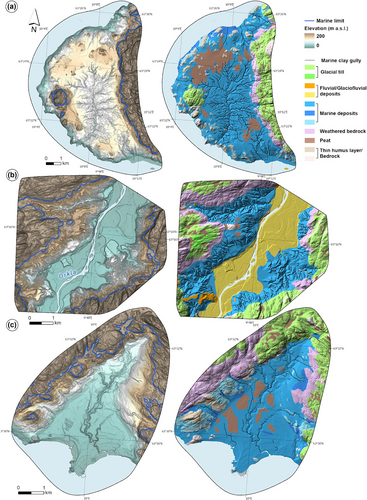
In this study, we address these issues by (1) exploring automated differentiation of intact and impacted gullies, (2) carefully choosing predictors that are typically used in manually mapping approaches of marine clay gullies, (3) testing the applicability of pre-trained models to blind-test areas on similar and different geological settings and (4) discussing the applicability of deep learning predictions for geomorphological mapping routines. We do so by assessing the automatic differentiation of gullies with high precision, using U-net architecture and fully convolutional neural networks (FCNNs). The selected study areas are in Romerike and in Trøndelag (Figures 1 and 2), where intact and impacted gully systems are found in different geological and geomorphological settings. We evaluate the predictions statistically by (a) calculating precision, recall and F1 score with ground truth data and (b) by comparing the predictions to a reference vector line dataset (Christoffersen et al., 2021; van Boeckel et al., 2022).

2 STUDY AREAS
The study areas represent different marine clay landscapes in two regions: in Romerike, South-East Norway, divided into Romerike North and Romerike South (Figure 1b), and in Mid-Norway, comprising of Byneset, Orkdal and Stadsbygd (Figure 2). All study areas are located below the marine limit, representing a modelled elevation of the highest relative sea level after deglaciation (Høgaas et al., 2022). The marine limit varies throughout the country; in South-East Norway, the marine limit reaches up to 220 m a.s.l., and in Mid-Norway, it reaches up to 190 m a.s.l. (NGU, 2024). The vast majority of the raised marine fine-grained deposits, hosting the marine clay gullies, are found below this limit.
All the study areas comprise large raised marine clay deposits, reflecting a near-horizontal surface of the old seabed before the inception of gully and river erosion. This near-horizontal surface can be regarded as a reference surface for estimating erosion depth in gullies and differs in elevation above sea level for each study area. Therefore, the base level of erosion along gullies is located at different elevations but is also controlled by bedrock, rivers, or the sea. An overview of the different characteristics of each study area and how the different areas have been involved in this study is shown in Table 1. More detailed descriptions of the different study areas are given below.
| Study area | Landscape characteristics | Usage | Reference data |
|---|---|---|---|
| Romerike South | Large flats of fine-grained marine deposits incised by large parallel and dendritic gully networks | Training and testing. Predictions evaluated with reference data | Vector lines (van Boeckel et al., 2023) |
| Romerike North | Large flats of fine-grained marine deposits incised predominantly dendritic gully networks | Blind-test area, predictions evaluated with reference data | Vector lines (van Boeckel et al., 2022) |
| Byneset | Large flats of fine-grained marine deposits incised by a few large dendritic gully networks | Blind-test area, predictions evaluated with reference data | Vector lines (NGU, 2024) |
| Orkdal | Narrow fjord valley with large fluvial plains and closely spaced gullies | Blind-test area, predictions evaluated with reference data | Vector lines (NGU, 2024) |
| Statsbygd | Low and flat-lying marine deposits with short and shallow gullies | Blind-test area, predictions evaluated with reference data | Vector lines (Christoffersen et al., 2021) |
Romerike and Byneset are characterised by bedrock hills protruding through large flats of fine-grained marine deposits (Figures 1b and 2a). These deposits have widely been incised by large, often dendritic networks of gullies and/or substantial quick-clay landsliding. The extensive networks of gullies vary in length from nearly a kilometre up to 10 km and depths between a few metres up to 40 m. Romerike has two large rivers, Glomma and Vorma. The gullies along these river systems, adjacent to the fluvial bars and plains, are relatively parallel and straight, oriented perpendicular to the main river, with less dendritic branching. Romerike also has four other smaller river systems, and large gully networks are connected to three of them. The main stream in Byneset is small, and its outlet is on bedrock that acts as the erosional basis.
Orkdal is a relatively narrow fjord valley with steep bedrock sides. Along the valley runs a large meandering river, Orkla, with fluvial plains and terraces in the valley bottom. The marine clay deposits are exposed at higher elevations on the valley sides but lie stratigraphically beneath the fluvial deposits in the valley bottom (Figure 2b). The gullies in Orkdal are steep, closely spaced and oriented perpendicular to the main river. Here, the gullies are relatively short, with only a few branched into networks and longer than 1 km.
Stadsbygd has one main, small stream in relatively flat-lying marine deposits confined by bedrock and with an outlet in the sea. The stream has only a few attached short and shallow gullies with depths of less than 10 m (Figure 2b).
3 METHODS
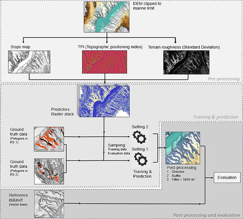
We aimed to train our models to identify and delineate gullies using a minimum number of predictor variables, comprising solely terrain derivatives and ground truth data from Romerike S. We then assessed the performance of our models to sampled ground truth data for evaluation and compared our predictions to reference datasets, see Figure 3 and Table 1.
3.1 Data input and preparation
3.1.1 Data preparation—ground truth data
Marine clay gullies were digitised manually and prepared as ground truth data for training the model. The landforms were digitized using light detection and ranging (LiDAR) data, orthophotos provided by Kartverket (the Norwegian Mapping Authority) and existing Quaternary geological maps (NGU, 2024). The landforms were mapped with a minimum size of 2500 m2. The shape of many individual gullies, or sections of more extensive gully networks, is partly impacted by human activity, often as a result of agricultural levelling and ploughing, and filling of construction material (Erikstad, 1992; van Boeckel et al., 2022). Because the morphology of impacted, often smoothened, gullies differ to such an extent from the unimpacted, steep and V-shaped gullies, we divided the ground truth dataset into two categories: sharp and smoothened gullies.
The width of sharp gullies scales with length but is typically less than 100 m wide and rarely exceeds 200 m. The slopes of both flanks are steep (>20°), often symmetrical, with abrupt boundaries to a surrounding near horizontal surface (Figure 4f). The centreline along the base of the gully is gradually inclined with deeper incisions in the downstream direction. In contrast, smooth gullies are typically wider, ranging between 100 and 250 m, irrespective of the length of the gullies. The boundary of smooth gullies is more gradual, with shallow slopes along the flanks (<10°). The base has a lower relative topography compared with sharp gullies, in respect to the surrounding surface elevation. Due to levelling and/or infill of material, the base of smooth gullies can sometimes be undulating in the long-profile direction (Figure 4f).
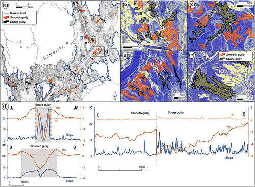
Because the morphology of gullies also differs from near parallel gullies to dendritic gully systems, we depicted subsets of training data that covered both types of gully networks in the regions RS 1 and RS 2 in Romerike South (Figures 3 and 4). In order to test the amount of training data needed to predict gullies, we used two different settings: Setting 1, which included training data of the whole Romerike South, including ground truth data from RS 1 and RS 2, and Setting 2, which only used training data from RS 1 (Figures 3 and 4). In total, 186 smooth and 147 sharp (Table 3) gullies randomly spread with different sizes were used for training.
3.1.2 Predictor variables—terrain derivatives from DEM
To target the above-mentioned morphological characteristics of marine clay gullies, we chose to use solely terrain derivatives describing the relative topography as predictor variables. We calculated the terrain derivatives from a high-resolution digital elevation model (DEM), derived from LiDAR, accessed January 2023 at https://hoydedata.no. The DEM is clipped to the area below the marine limit (Høgaas et al., 2022) and has a spatial resolution of the DEM 1 m with a vertical accuracy of approximately 0.1 m (Terratec, 2022). The terrain derivatives comprised of slope, TPI, and terrain roughness (TR) were stacked into one composite band; accordingly, see Figure 3. We used a moving window of 100 m for calculating TPI with the tool ‘DiffFromMeanElev’ using WhiteboxTools (Lindsay, 2014) and a moving window of 5 m for calculating the TR using the standard deviation of the surrounding topography (Grohmann, Smith, & Riccomini, 2009).
Initial test runs also included additional categorical data, such as land-use maps Arealressurskart (1: 5 000) (AR5) (Ahlstrøm, Bjørkelo, & Fadnes, 2019), surficial deposit maps in 1:50 000 (NGU, 2024) and continuous elevation data. Due to unsuccessful predictions of gullies of the pre-trained model for the blind-test areas, and because the scope of this study was to apply the pre-trained model to other regions, we decided to drop these predictor variables for further analysis which will not be presented in our results section.
3.2 Method and evaluation
3.2.1 Semi-automated mapping
We used a convolutional neural network (CNN) to gullies using training data consisting of predictor variables (slope, TPI and TR) and ground truth data. Models based on CNN can distinguish patterns exceptionally well in applications that deal with image data (Chen et al., 2019; Zaidi et al., 2022). Convolutions are matrix calculations based on a moving window, usually using 3 × 3 cells, to compile geospatial information into classified tiles (Albawi, Mohammed, & Al-Zawi, 2017). The spatial dimension of the classified tiles is crucial; therefore, we apply U-net (Ronneberger, Fischer, & Brox, 2015) and CNN architecture for semantic segmentation and pixel-based classification (Prakash, Manconi, & Loew, 2021; Zhang, Zhang, & Du, 2016). We used the backbone ResNet34 to create the UnetClassifier base, using ArcPy libraries to build a dynamic U-Net. U-Net is known for being fast, effective and precise in segmentation, recognising objects based on local information in the ground truth (Leng et al., 2019). This approach requires two types of data sources for training: ground truth data, with vector-based manually mapped features aimed to be predicted, and terrain derivatives used for recognising these features (Nodjoumi et al., 2023). To train robust models (Shelhamer, Long, & Darrell, 2017; Ye, Ni, & Yi, 2017), we used training datasets for Settings 1 and 2 containing both a raster stack of terrain derivatives and classified ground truth polygons for the corresponding areas; see also Figure 3. After testing the training data with different numbers of classified tiles, we found that 20 000 randomly generated samples, exported as classified tiles, performed the best to train the model. The randomly generated samples were exported as classified tiles using an Image Analyst licence (‘Export Training Data for Deep Learning’) from ArcGIS Pro (ArcGIS Pro, 2022). The most suitable classified tile size in our case was 256 × 256 pixels, and in order to have 50% overlap in each sample tile when creating the following image chips, the stride, which describes the distance of movement in the x- and y-direction, was set to be 128 × 128 pixels. The entire process of training, evaluating and exporting the model was conducted using Jupyter Notebook and ArcPy libraries. During the training process, an input image in the form of classified tiles flows through the CNN network that recognizes it with a set of trainable kernels, resulting in a group of feature maps (Liu, 2018). The models were trained for 50 epochs. To avoid overfitting, we set an early stopping parameter when the training did not improve after 10 epochs. We also applied the Adam optimizer (Kingma & Ba, 2015; Malik et al., 2021). The other parameters were maintained at their default values. The trained model was saved as a ‘Deep Learning Package’(‘.dpk’ format), which is the standard format used to deploy deep learning models on the ArcGIS Pro platform and can be used further as a pre-trained model (ESRI, 2023; Ma & Mei, 2021; Miranda & Von Zuben, 2015). The trained models were then used to predict gullies in the other study areas for the blind test (Figures 1b and 2).
3.2.2 Evaluation
The resulting predictions of smooth and sharp gullies were evaluated quantitatively by comparing pixels of the sampled ground truth data of gullies to the automated gullies' predictions of the same areas. We calculated metric precision, recall and F1 score metrics to evaluate the performance of the two proposed models. Precision is a measure of how many of the positive predictions are made correctly (true positives) (Table 2a), while recall is a measure of how many of the positive cases were correctly predicted, over all the positive cases in the data. F1 score is a measure combining both precision and recall. A satisfactory F1 score means that there are low false positives and low false negatives. An F1 score is considered solid with a value close to 1 (Table 2b) (Lipton, Elkan, & Naryanaswamy, 2014).
| (a) | |||
|---|---|---|---|
| Prediction | Actual value | Type | Explanation |
| 1 | 1 | True positive (TP) | Predicted positive and was positive |
| 0 | 0 | True negative (TN) | Predicted negative and was negative |
| 1 | 0 | False positive (FP) | Predicted positive but was negative |
| 0 | 1 | False negative (FN) | Predicted negative but was positive |
| (b) | |
|---|---|
| Metric | Formula |
| Precision | |
| Recall | |
| F1 score | |
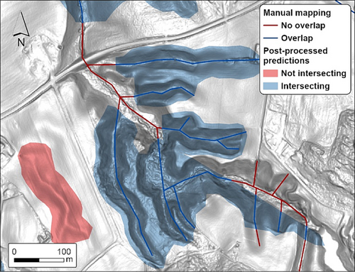
When trained properly, pre-trained models can be used for similar problems in similar settings to save time and reduce the need for more ground truth data (Ma & Mei, 2021; Tehrani et al., 2022). For this reason, we test our pre-trained models' applicability to the four blind-test areas: Romerike N, Byneset, Orkdal and Stadsbygd (Figures 1 and 2). Here, we regard Romerike N and Byneset to have a similar geological setting with large networks of dendritic gullies. In Orkdal and Stadsbygd, the geological setting is different, with shorter, often shallower and more individual gullies. We compare the predictions in all study areas with a reference dataset comprising manually mapped gullies as vector lines from the Norwegian geological survey (Christoffersen et al., 2021; van Boeckel et al., 2022) (Figures 1c and 2 and Table 1). First, we post-processed the predicted delineations to remove noise, which therefore readily can be incorporated into manual geomorphological mapping routines. The post-processing comprised (1) transforming the pixels into vector shapes, (2) buffering and dissolving the vector shapes with a 5 m radius, and (3) applying a filter by removing polygons smaller than 5000 m2. Then, we compared the post-processed predictions using an overlay and intersect analysis to calculate length-weighted overlap and coverage of intersecting gullies. The latter represented the relative surface area of post-processed predictions intersecting with the reference dataset. We regard the intersecting predictions as true positives, which we can then use as a first-order indication of the agreement between post-processed predictions and the reference dataset. The length-weighted overlap represented the relative length of the vector lines overlapping with the post-processed predictions. The cumulative lines that did not overlap with the post-processed predictions can be regarded as an indicator of false negatives (Figure 5). We note that comparing the reference dataset with post-processed predictions does not give any information about the accuracy of the delineation of the landforms, which was done visually.
4 RESULTS
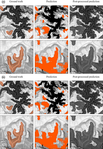
In this section, we present the performance of the U-net model in Romerike S by applying two data settings (Settings 1 and 2) using Jupyter Notebook and ArcPy libraries environment. The quantitative evaluation of the sampled pixels between ground truth data and predictions is presented in Table 3. Statistically, we can see higher precision (0.75–0.82), recall (0.69–0.73) and F1 score (0.72–0.74) for sharp gullies. On the other hand, smooth gullies have a tendency to achieve lower scores for precision (0.70–0.72), recall (0.66–0.72) and 0.68–0.72 for the F1 score (Table 3). Our results show that by using the same amount of ground truth data (20 000) but from a more extensive and more diverse study area, the performance of Setting 1 (Figure 1) only increased slightly for sharp gullies but decreased for smooth gullies, with an F1 score of +0.02 and −0.04, respectively.
| Setting 1 | Setting 2 | |||
|---|---|---|---|---|
| Smooth gullies | Sharp gullies | Smooth gullies | Sharp gullies | |
| GTPs | 186 | 147 | 95 | 47 |
| Precision | 0.70 | 0.75 | 0.72 | 0.82 |
| Recall | 0.66 | 0.73 | 0.72 | 0.69 |
| F1 | 0.68 | 0.74 | 0.72 | 0.72 |
- Abbreviation: GTPs, ground truth polygons.
Even though the statistics show minor differences in the overall performance using the different data settings, visual inspection reveals that the different models pick up different sections along the same gullies. This can also be observed when comparing the predictions to the reference datasets. When combining the predictions of Settings 1 and 2, the length-weighted overlap and coverage of intersecting gullies score slightly higher compared with the values by only using Setting 2, increasing the respective average scores with +10% and +2.4% (Table 4).
| Setting 2 | Settings 1 and 2 | |||||
|---|---|---|---|---|---|---|
| Predictions (nr.) | Coverage of intersecting gullies | Length-weighted overlap | Predictions (nr.) | Coverage of intersecting gullies | Length-weighted overlap | |
| Romerike S | 2117 | 82.8% | 67.8% | 1918 | 87.4% | 70.5% |
| Romerike N | 1245 | 94.7% | 76.6% | 954 | 94.1% | 86.1% |
| Byneset | 175 | 91.7% | 64.5% | 160 | 91.4% | 72.7% |
| Orkdal | 120 | 94.9% | 55.1% | 105 | 94.1% | 67.2% |
| Stadsbygd | 59 | 71.2% | 38.4% | 72 | 80.2% | 56.1% |
The next step was to compare the predictions of the pre-trained models to the reference datasets in Romerike S and the four blind-test areas: Romerike N, Byneset, Orkdal and Stadsbygd (Figures 1 and 2 and Table 4). We applied both pre-trained models (Settings 1 and 2) to all the study areas and post-processed the predicted pixels, as explained in Section 3.2.2. The first category of blind-test areas, Byneset and Romerike N, with a similar geological setting as Romerike S, show promising results scoring 91.7% and 94.7% for coverage of intersecting gullies and 64.5% and 76.6% for length-weighted overlap, respectively. These values increased slightly when combining the post-processed predictions of Settings 1 and 2 (Table 4). The blind-test areas Stadsbygd and Orkdal scored poorly in length-weighted overlap with 38.4% and 55.1%, respectively, when only using the post-processed products of Setting 2. The low length-weighted overlap values indicate that the pre-trained models did not pick up many vector lines from the reference dataset. The coverage of intersecting gullies scored relatively high (>71%) for all the blind-test areas, which indicates that the post-processed predictions of the pre-trained models largely managed to successfully identify the gullies.
5 DISCUSSION
5.1 Automated differentiation of intact and impacted gullies
The delineation of landforms is the fundamental process of mapping the spatial extent and condition of landscape change, which conventionally is performed manually using high-resolution optical remote-sensing images or LiDAR data. Our results show that using only three terrain derivatives and 142 manually mapped gullies (Setting 2), the U-net model successfully predicted and differentiated intact sharp gullies from impacted smooth gullies. Quantitative pixel evaluation of sampled ground truth data revealed that doubling the ground truth data (Setting 1) only slightly improved the F1 score for sharp gullies (+0.02) but decreased for smooth gullies (−0.04). Overall, both automated identification models revealed promising results in differentiating gullies impacted by agricultural levelling from intact gullies, as also seen in Roy & Saha (2022).
5.2 The minimal amount of predictors
For the blind-test areas, the best predictions were achieved using predictors indicative of relative elevation, for example, the terrain derivatives slope, TR and TPI, as opposed to absolute elevation from DEMs. We explain this by the fact that the gullies are found in raised marine fine-grained deposits at varying elevations between the study areas (Figures 1 and 2). Because the model was trained on ground truth data located at elevations between approximately 100 and 180 m a.s.l., the pre-trained model was unable to detect gullies at lower elevations. We, therefore, stress that using elevation data as a predictor should be used with caution when predicting blind-test areas.
Unlike similar studies delineating gullies with the usage of over a dozen independent predictors (Band et al., 2020; Setargie et al., 2023), we show that a promising delineation of gullies can be achieved by only using three predictor layers derived from high-resolution elevation data. Although we recognize that adding additional predictor variables, such as curvature- or slope of slope terrain derivatives and categorial land-use maps, could potentially improve the performance of our models, we argue that having few predictors makes our approach more accessible and applicable in other areas for future mapping.
5.3 The applicability of pre-trained models to blind-test areas
The robustness of a model increases when successful predictions are not limited to trained areas but also manage to predict in blind-test areas for other regions (Sarker, 2021). As we do not have ground truth data of our blind-test areas, we rely on overlay analysis between the vector-line reference dataset with post-processed predictions. Our results show that the post-processed predictions broadly intersect with the reference dataset (>71.2%). If we only regard the blind-test areas with similar geological settings, namely, Romerike N and Byneset, the coverage of intersecting gullies increases to >91.7%, indicating that the model manages to accurately identify gullies. Similarly, Romerike N and Byneset score significantly higher in length-weighted overlap compared with Orkdal and Stadsbygd, reflecting that large stretches of the reference dataset overlap with the pre-trained models. The difference in geological setting can explain the discrepancy of lower length-weighted overlapping values for Orkdal and Stadsbygd. In these areas, the gullies are much shorter and less branched into networks compared with the gullies used in the ground truth dataset. Future incentives to train the model specifically for these settings or to include them in the training dataset might increase the model's performance.
We noticed that the delineation of the predictions was improved by using the combined predictions of Settings 1 and 2. This improved performance is also reflected by higher length-weighted overlap values for all blind-test areas, increasing the length-weighted overlap by an average of +10%. Similar to the studies of Arabameri et al. (2021) and Roy and Saha (2022), which used ensemble models for forecasting areas vulnerable to gully erosion, our findings confirm that the combined products of the pre-trained models increase the overall delineation of the gullies.
5.4 Applicability of DL in geomorphological mapping
One of the advantages of using automated approaches compared with manual mapping is that the automatic delineation of landforms can be evaluated quantitatively against ground truth data. For example, predictions can be evaluated by positively identified pixels (e.g. Setargie et al., 2023) and positively identified vector lines (e.g. Band et al., 2020). Even though quantitative evaluations can give satisfactory results, there is little information about the correctness of the delineation of the predicted gullies. A gully can, for example, be identified with a pixel accuracy of 75%, but this does not necessarily mean that the outer extent of the predicted gully corresponds to the actual landform. As manual mapping routines often involve the delineation of individual landforms, having an inaccurate outer delineation still requires substantial adjustments to be implemented to satisfy the prerequisites for usage in geomorphological maps. We found that post-processing the pixel-based predictions into coherent polygons and reducing noise with a minimum size filter significantly increased the applicability of the product for mapping routines, see also Figure 6. We point out that the post-processing of prediction delineations should be considered when implementing automated approaches in manual mapping routines.
6 CONCLUSION
Development in computing, deep learning algorithms and increased availability of high-resolution and free data have the potential to automate many mapping problems in Earth sciences. However, its application in differentiating and delineating landforms in mapping routines using deep learning techniques has not been thoroughly investigated. We contribute by exploring the automated differentiation of intact (sharp) and impacted (smooth) gullies with high precision using the combination of the deep learning FCNN model with only three terrain derivatives (slope, TR and TPI). Our best model achieved a precision score of 0.82 and 0.72 for sharp and smooth gullies, respectively. Our pre-trained models successfully predicted gullies in blind-test areas, scoring >70% length-weighted overlap and >82% coverage of intersecting gullies for regions with similar geological settings. We find that combining model predictions, along with processing the predictions, increases the agreement between automated delineations and reference datasets. We therefore stress the importance of post-processing steps to enhance the applicability of deep learning models in geomorphological mapping routines. The outcome of this research contributes towards better implementing automated approaches in manual mapping routines, as well as the development of monitoring systems for future landscape change.
AUTHOR CONTRIBUTIONS
Conceptualization: Alexandra Jarna Ganerød and Mikis van Boeckel. Methodology: Alexandra Jarna Ganerød and Mikis van Boeckel. Software: Alexandra Jarna Ganerød and Mikis van Boeckel. Validation: Alexandra Jarna Ganerød and Mikis van Boeckel. Formal analysis: Alexandra Jarna Ganerød and Mikis van Boeckel. Investigation: Alexandra Jarna Ganerød and Mikis van Boeckel. Resources: Alexandra Jarna Ganerød, Mikis van Boeckel and Inger-Lise Solberg. Data curation: Alexandra Jarna Ganerød and Mikis van Boeckel. Writing—original draft preparation: Alexandra Jarna Ganerød, Mikis van Boeckel and Inger-Lise Solberg. Visualization: Alexandra Jarna Ganerød and Mikis van Boeckel. All authors have read and agreed to the published version of the manuscript.
ACKNOWLEDGEMENTS
We are grateful to all those with whom we have had the pleasure to work during this and other related projects connected to the topic. The copy read by Danielle Robert benefited this manuscript. Thank you to Gabriela Spakman-Tánásescu for introducing ArcGIS Pro and deep learning possibilities and the DEEP: Norwegian Research School for Dynamics and Evolution of Earth and Planets.
Open Research
DATA AVAILABILITY STATEMENT
The source code is available for download here: https://github.com/alexandra-jarna/Ravines-Norway. Programme language: Python. Software required: data preparation (ArcGIS Pro/QGIS). Pretrained models are available for download here: https://github.com/alexandra-jarna/Ravines-Norway/blob/main/pre-trained-models.


