Prediction of the water level at the Kien Giang River based on regression techniques
Abstract
Model accuracy and runtime are two key issues for flood warnings in rivers. Traditional hydrodynamic models, which have a rigorous physical mechanism for flood routine, have been widely adopted for water level prediction in river, lake, and urban areas. However, these models require various types of data, in-depth domain knowledge, experience with modeling, and intensive computational time, which hinders short-term or real-time prediction. In this paper, we propose a new framework based on machine learning methods to alleviate the aforementioned limitation. We develop a wide range of machine learning models such as linear regression (LR), support vector regression (SVR), random forest regression (RFR), multilayer perceptron regression (MLPR), and light gradient boosting machine regression (LGBMR) to predict the hourly water level at Le Thuy and Kien Giang stations of the Kien Giang river based on collected data of 2010, 2012, and 2020. Four evaluation metrics, that is, R2, Nash–Sutcliffe efficiency, mean absolute error, and root mean square error, are employed to examine the reliability of the proposed models. The results show that the LR model outperforms the SVR, RFR, MLPR, and LGBMR models.
1 INTRODUCTION
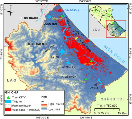
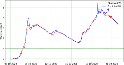
The Kien Giang River, one of two major tributaries within the Nhat Le River system, flows through the Le Thuy and Quang Ninh districts in Quang Binh province (Vietnam) (Figure 1). Spanning approximately 69 km in total length (Ly et al., 2013), this area has been known as a “flood navel” since the formation of Le Thuy and Quang Ninh topography. During the historical flood in October 2020, more than 50,000 houses at the foothills of the Truong Son mountain range were submerged, and thousands of villages and hamlets were isolated. The flood peak at the Le Thuy station reached 4.88 m, exceeding the warning level III and 0.97 m higher than the historical flood peak in 1979.
Accurately forecasting the river water level is critical for early flood warning and flood disaster mitigation. In general, there are two main approaches to predict the water level. The former relies on physically based models, such as the MIKE HYDRO River, HEC-HMS, SOBEK, and EFDC. Although these models have high accuracy, they typically require a variety of datasets, including topographic, meteorological, and hydrological data, and intensive computational time for model simulation. Therefore, physically-based models are unsuitable for short-term and real-time prediction. Moreover, the development of a physically based model frequently demands in-depth knowledge and expertise in the hydrological field (Atashi et al., 2022).
An alternative approach is a data-driven model that collects and analyzes the statistical relationship between input and output data. This approach can help overcome the limitations mentioned above of the physically based model. The machine learning (ML) model has been used for flood forecasting since the 1990s and is one of the most popular frameworks utilized in the data-driven method. Recent studies suggest that ML can be a powerful tool for flood forecasting because it can be built quickly and effortlessly without understanding the underlying process. In addition, other main advantages of ML models are the shorter computational time, faster calibration and validation, and easier usage compared to the physically based models (Mekanik et al., 2013).
To our knowledge, no previous studies have applied the ML approach to predict river water levels for the Quang Binh province. The goal of our study is to apply regression methods, including linear regression (LR), support vector regression (SVR), random forest regression (RFR), multilayer perceptron regression (MLPR), and light gradient boosting machine regression (LGBMR) to predict water level at the Le Thuy and the Kien Giang stations.
2 METHODOLOGY AND DATA COLLECTION
2.1 Regression methods
2.1.1 LR
LR is a machine learning algorithm based on supervised learning, which models a target prediction value based on independent variables. Different regression models differ based on the kind of relationship between the dependent and independent variables they are considering and the number of independent variables getting used. The regression's dependent variable can be referred to as an outcome variable, a criterion variable, an endogenous variable, or a regressand. Respectively, the independent variable can be referred to as an exogenous variable, a predictor variable, or a regressor.
2.1.2 SVR
2.1.3 RFR
- 1.
On the basis of the bootstrap method, a subset of samples is randomly produced with replacements from the original data set.
- 2.
These bootstrap samples are employed to construct regression trees. The optimal split criterion is used to split each node of the regression trees into two descendant nodes. The process on each descendant node is continued recursively until a termination criterion is fulfilled.
- 3.
Each regression tree provides a predicted result. Once all of the regression trees have reached their maximum size, the final prediction is determined as the average of the results from all of the regression trees:
2.1.4 MLPR
2.1.5 LGBMR
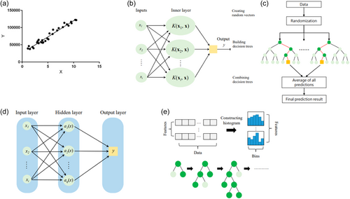
LGBMR uses four main algorithms to improve computational efficiency and prevent overfitting: gradient-based one-side sampling (GOSS), exclusive feature bundling (EFB), a histogram-based algorithm, and a leaf-wise growth algorithm (He et al., 2022; Ke et al., 2017). As shown in Figure 2d, the leaf-wise growth algorithm allows the identification of the leaf node with the largest split gain while preventing overfitting. In addition, LGBMR adopts the histogram-based decision tree algorithm to divide continuous floating-point features into a variety of intervals to reduce the computational power required for prediction. Moreover, GOSS and EFB are used to reduce the number of samples for accelerating the training process of LGBMR.
2.2 Evaluation metrics
-
Coefficient of determination (R2)
() -
Nash – Sutcliffe efficiency (NSE)
() -
Mean absolute error (MAE)
() -
Root mean square error (RMSE)
3 RESULTS AND DISCUSSION
In this study, we predict water levels at the Le Thuy and Kien Giang stations using five regressive machine learning models. We employ six evaluation metrics R2, NSE, MAE, RMSE, PR, and to assess the models' performance. Accordingly, the ideal input data set parameters and the most effective machine learning strategy for this issue are selected. Regressive machine learning models are installed using the Python 3.7 environment.
3.1 Study area and data
The Nhat Le River basin, which has a total area of 2612 km2, includes three main tributaries: Kien Giang, Long Dai, and Nhat Le (Figure 1). Three medium-sized irrigation reservoirs, An Ma, Cam Ly, and Rao Da, have a small flood capacity of 22.1, 6.9, and 11.6 million m3, respectively. Other reservoirs have smaller capacities, so the impact of their operation on downstream water levels is negligible.
In this study, we use hourly rainfall and water level data collected from three stations, namely Kien Giang, Le Thuy, and Dong Hoi. The data set contains the flood season of 2010, as weel as the whole year of 2012 and 2020. We split the data set into two parts: training data from 2010 to 2012 (10,297 samples), and testing data from 2020 data (8785 samples).
3.2 Input data set to predict water level at Le Thuy and Kien Giang stations
We use the data set of hourly water levels and rainfalls recorded at three stations (Kien Giang, Le Thuy, and Dong Hoi) in the years 2010, 2012, and 2020. Through previous research and analysis, it is discovered that the water level at a station is influenced by previous rainfall and water levels at that station and nearby stations. One problem is determining the length of past input data to acquire the highest performance. This study also employs hourly data, allowing us to predict the water levels for 1, 6, and 12 h-ahead. To improve accuracy, we experiment with integrating predicted rainfall data from hydro-meteorological stations for the following 1, 6, and 12 h as additional features. The following sections will present these experiment's findings.
Choosing the number of time lags and time leads
In which , are the forecast water levels at Le Thuy and Kien Giang stations, respectively, t is the present time, t + h is the predicted time (h = 1, 6, or 12 h). are the rainfalls at the three stations at present, in the past and the future (predicted rainfall), is the number of time lags, are the water levels at three stations (Le Thuy, Kien Giang, and Dong Hoi) at present and in the past.
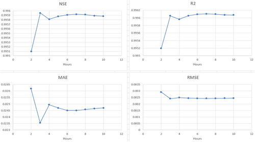
With the LR model, the number of time lags is selected between 1 and 10 h (k = 1–10) to predict the water level for the next six time leads (h = 6 h) at the Le Thuy station. The results show that the use of data from 2 to 10 h ago to predict the water level for the next 6 h yields good result with the values of R2 and NSE are both above 0.99. Especially, at k = 3, all four metrics demonstrate the best performance, with MAE and RMSE error of 2.35 and 0.25 cm, respectively. In addition, the peak error in the 2020 flood, Ep is 0.7 cm when k = 3. Therefore, we decided to select the 4-day input data set (at time t, t − 1, t − 2, and t − 3) to predict the water level at 1, 6, and 12 h (h = 1, 6, 12) in the following section. (Figure 3).
3.3 Prediction results of water levels in Kien Giang and Le Thuy
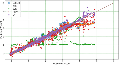
In this experiment, the water level at Le Thuy station was predicted using five regression models: LR, RFR, SVR, MLPR, and LGBMR. The scatter plot (Figure 4) compares the models' water level predictions with a 6h time lead. We can observe that the MLPR model underperforms compared to the the LR, RFR, and LGBMR models, while the SVR model performs the worst as the distribution of points furthest from the 1:1 line. When the water level is below warning level III (H = 2.7 m), the RFR and LGBMR models produce results close to the 1:1 line. However, the forecast value of the RFR and LGBMR models is also lower than the observed value as they fail to estimate the flood's peak water level.
Tables 1 and 2 show the details of the assessments of the capacity to replicate water levels at the Le Thuy and Kien Giang stations, respectively. Observed water level and rainfall data in 2010 and 2012 and predicted rainfall are used as training data at three locations: Kien Giang, Le Thuy, and Dong Hoi. The model's output is the water level at Le Thuy and Kien Giang for the following 1, 6, and 12 h. The 2020 data set was used to test the model. The SVR model performs poorly, while the three models LR, RFR, and LGBMR, give good results in terms of NSE, R2, MAE, and RMSE value.
| Model | Time lags (h) | NSE | R2 | MAE (m) | RMSE (m) | PE (m) Observed peak: 4.88 m |
|---|---|---|---|---|---|---|
| LR | 1 | 0.9999 | 0.9999 | 0.0045 | 0.0001 | 0.0226 |
| 6 | 0.9960 | 0.9961 | 0.0236 | 0.0024 | 0.2143 | |
| 12 | 0.9869 | 0.9876 | 0.0422 | 0.0078 | 0.3933 | |
| RFR | 1 | 0.9943 | 0.9952 | 0.0103 | 0.0034 | 1.0807 |
| 6 | 0.9858 | 0.9875 | 0.0334 | 0.0085 | 1.2022 | |
| 12 | 0.9732 | 0.9733 | 0.0564 | 0.0159 | 1.1532 | |
| SVR | 1 | 0.8903 | 0.8976 | 0.0774 | 0.0652 | 2.4954 |
| 6 | 0.8261 | 0.8318 | 0.0813 | 0.1034 | 3.8098 | |
| 12 | 0.7943 | 0.8031 | 0.0989 | 0.1223 | 3.7720 | |
| MLPR | 1 | 0.9938 | 0.9939 | 0.0198 | 0.0037 | 0.1666 |
| 6 | 0.9808 | 0.9832 | 0.0420 | 0.0114 | 0.7417 | |
| 12 | 0.9628 | 0.9635 | 0.0581 | 0.0221 | 0.6911 | |
| LGBMR | 1 | 0.9916 | 0.9926 | 0.0136 | 0.0050 | 1.1828 |
| 6 | 0.9848 | 0.9856 | 0.0345 | 0.0090 | 1.1766 | |
| 12 | 0.9763 | 0.9764 | 0.0529 | 0.0141 | 1.1107 |
- Note: The significance of bold which is the LR model gives the best result.
- Abbreviations: LGBMR, light gradient boosting machine regression; LR, linear regression; MLPR, multilayer perceptron regression; RFR, random forest regression; SVR, support vector regression.
| Model | Time lags | NSE | R2 | MAE (m) | RMSE (m) | PE (m) Observed peak: 14.66 m |
|---|---|---|---|---|---|---|
| LR | 1 | 0.9983 | 0.9983 | 0.0104 | 0.0011 | 0.2215 |
| 6 | 0.9363 | 0.9385 | 0.0788 | 0.0437 | 1.3489 | |
| 12 | 0.8908 | 0.8983 | 0.1143 | 0.0748 | 0.2867 | |
| RFR | 1 | 0.9932 | 0.9936 | 0.0138 | 0.0047 | 2.0925 |
| 6 | 0.9394 | 0.9407 | 0.0688 | 0.0416 | 2.7378 | |
| 12 | 0.8912 | 0.8926 | 0.1064 | 0.0746 | 3.6833 | |
| SVR | 1h | 0.8243 | 0.8397 | 0.0977 | 0.1206 | 7.2003 |
| 6 | 0.7405 | 0.7604 | 0.1189 | 0.1779 | 7.2043 | |
| 12 | 0.7008 | 0.7273 | 0.1482 | 0.2051 | 7.1874 | |
| MLPR | 1 | 0.9770 | 0.9792 | 0.0498 | 0.0158 | 0.6581 |
| 6 | 0.8336 | 0.8637 | 0.0897 | 0.1141 | 5.0895 | |
| 12 | 0.6689 | 0.7865 | 0.1516 | 0.2269 | 0.6804 | |
| LGBMR | 1 | 0.9870 | 0.9877 | 0.0235 | 0.0089 | 2.5578 |
| 6 | 0.9499 | 0.9502 | 0.0688 | 0.0343 | 2.0842 | |
| 12 | 0.9305 | 0.9311 | 0.0960 | 0.0476 | 2.7698 |
- Note: The significance of bold which is the LR model gives the best result.
- Abbreviations: LGBMR, light gradient boosting machine regression; LR, linear regression; MLPR, multilayer perceptron regression; RFR, random forest regression; SVR, support vector regression.
Forecasting is crucial for flood disaster mitigation and prevention. One of the requirements to determine a model's validity is accurate reporting of flood peaks and time to peak. With NSE and R2 greater than 0.99, RMSE of 0.007 and MAE of 0.11, and especially the error of flood peak less than 8% (equivalent to 39.3 cm in case h = 12 h at Le Thuy station), and 2% (i.e., 2.87 cm in case h = 12 h at Kien Giang station), and ∆t = 1 h. The results demonstrate that the LR model gives the best result. First, the results of the LR model are shown in Tables 1 and 2. Second, the relationship between rainfall and the water level is linear. Third, the water level of the stations (Le Thuy, Kien Giang, Dong Hoi) is the linear influence.
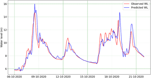
Figures 5 and 6 show the actual water level measured and the predicted water level generated by LR model with time lead 6h during the historic flood from October 6, 2020, to October 21, 2020, at two stations (Le Thuy and Kien Giang). We can observe that the predicted line and measured line are very close to one another. However, the results of the linear regression model are still unreliable, particularly at the flood peak. The method of employing input data, such as the water level in Dong Hoi, may be to blame for this. Due to the high tide impacts on Dong Hoi water level, the water level process curve changes occasionally. The water level in Le Thuy thus tends to fluctuate similarly to the water level in Dong Hoi when training the data, despite the possibility that the water level in Le Thuy is mostly unaffected by high tides. To further improve the model prediction accuracy, more research should take a variety of other variables into account, such as the geography of the location, ground cover, and initial moisture conditions.
4 CONCLUSIONS
In this study, we have developed models to predict the water level at the Le Thuy and Kien Giang stations on the Kien Giang River using LR, RFR, SVR, MLPR, and LGBMR regression techniques. The models are trained and validated using the hourly rainfall and water levels datasets at three stations in 2010, 2012, and 2020. The study's findings indicate that the best water level prediction result at the Le Thuy station at 6hrs ahead when using input data of hourly rainfall and water level in the period [t − 3, t], as well as the predicted rainfall at three hydrometeorological stations in the area. The model can forecast both the trough and peak of the water level. Evaluation metrics R2, NSE, MAE, and RMSE show that the application of the data-oriented model is feasible and reliable in predicting water levels in which the LR outperforms the other four regression methods.
In future studies, we will consider the addition of other inputs such as flows, tidal levels, rainfalls at nearby stations, or forecasted rain from the hydro-meteorological center stations (instead of using actual rainfall data measured at timestep t + 1), constructing water level forecasting models for hydrological stations and other “virtual” stations along the Kien Giang and Nhat Le rivers. In addition, other machine learning techniques, such as deep learning algorithms, will also be explored to enhance the accuracy of future water level forecasts.
ACKNOWLEDGMENTS
The authors would like to express their sincere gratitude for the support to complete this research. This research is supported by the Scientific Research and Technology Development Project at ministerial level, namely “Research on Digital Transformation in the flood warning methods for the community: an experimental flood warning system for Nhat Le river basin, Quang Binh province.”
ETHICS STATEMENT
None declared.
Open Research
DATA AVAILABILITY STATEMENT
The data that support the findings of this study are available from the corresponding author upon reasonable request.


