1 INTRODUCTION

In the past, vegetation in streams and rivers has been considered a source of flow resistance to be removed to increase the channel conveyance. Vegetation also plays a significant role in the interaction between aquatic ecosystems and river hydraulics (Ferro, 2019; Sandercock & Hooke, 2010) as it contributes to creating a wetland habitat for animal species, reduces bank erosion phenomena, and retains flow sediment transport (Errico et al., 2018, 2019). Modeling flow resistance in vegetated channels is useful to establish the propensity for flooding and design river management works aimed to flood mitigation (Green, 2005).

Many previous studies were developed for grass-like vegetation (Carollo et al., 2005, 2008; Errico et al., 2018, 2019; Ferro, 2019; Ghisalberti & Nepf, 2006; Ikeda & Kanazawa, 1996; Kouwen, 1988; Kouwen & Li, 1980; Kouwen & Unny, 1973; Kouwen et al., 1969; Kowobary et al., 1972; Termini, 2015) which is flexible, and is generally completely submerged as its bent vegetation height h_s is less than the flow depth h (Gourlay, 1970; Kouwen et al., 1969). For flexible vegetation, its configuration (erect, waving, prone) is due to the interaction between the hydrodynamic flow action and the stiffness characteristics of the vegetation elements (Ferro, 2019; Kouwen et al., 1969; Pasquino et al., 2018). The hydraulic behavior of a single vegetation type is also dependent on whether the plant elements are emergent, for h < h_s, or completely submerged (h > h_s). Furthermore, the flexible vegetation is characterized by the ratio h_s/H_v, named inflection degree, between the bent vegetation height h_s and the height H_v in the absence of flow. For rigid vegetation, the height h_s is coincident with H_v. The results of the investigations on grass-like vegetation (Carollo et al., 2005; Kouwen, 1992; Raffaelli et al., 2002; Wilson & Horritt, 2002) can be rarely applied to simulate riparian vegetation, which is frequently characterized by rigid, erect, and submerged or nonsubmerged condition. Vargas-Luna et al. (2016) analyzed the ability of this rigid cylinder analogy on reproducing vegetation's effects in all morphodynamic processes showing how cylinders well represent vegetation effects on channel width and bank-related processes. Previous investigations on flow resistance for rigid and nonsubmerged vegetation were generally carried out using laboratory flumes and artificial vegetation elements hydraulically similar to natural plants (Armanini et al., 2005; Chiaradia et al., 2019; Freeman et al., 2000; Rhee et al., 2008; Righetti & Armanini, 2002; Västilä et al., 2013; Wilson et al., 2003; Wu et al., 1999; Yagci et al., 2010).

The small-scale experimental studies on flow resistance in vegetated channels raise problems of similarity between models and prototypes. These small-scale experiments allow investigating the vegetation-flow interactions using controlled laboratory conditions even if scale problems related to flow hydraulics and vegetation conditions can occur. For this reason, the results obtained in flume investigations have to be carefully used to analyze natural conditions. On the contrary, full-scale measurements are useful to investigate in the field, with cumbersome experimental conditions, the relationship between vegetation properties (stiffness, stem concentration, branching, foliation) and flow conditions similar to the actual vegetation behavior (Florineth et al., 2003).

Notwithstanding numerous theoretical and experimental studies on flow resistance in vegetated channels have been carried out, and new estimate methods of the friction factor have been developed, classical hydraulic equations, such as those by Manning and Chezy (Govers et al., 2007; Nouwakpo et al., 2016; Powell, 2014; Strohmeier et al., 2014), are commonly applied to estimate open channel flow resistance. Manning's n or Darcy–Weisbach's f are frequently applied for vegetated channels (Yen, 1992):

()

in which V is the average cross-section velocity, u_* = is the shear velocity, g is the acceleration due to gravity, and s is the channel slope. Manning's coefficient has been generally applied to analyze field and flume measurements in vegetated channels, while f has been frequently used for developing theoretical analysis (Carollo et al., 2005; Ferro, 2019).

For improving the knowledge of flow resistance processes in vegetated channels, much research effort has been addressed to study the flow velocity distribution as its integration in the cross-section allows deducing a theoretical flow-resistance law (Ferro & Pecoraro, 2000; Ferro & Porto, 2018a).

Most of the recent studies of vegetated flows use a two-layer model for describing the velocity distribution: (i) a vegetation layer in which the flow velocity is assumed constant, and the drag resistance of a single vegetation element is considered; (ii) a surface layer in which a logarithmic distribution (Baptist et al., 2007; Cheng, 2011; Liu et al., 2008; Nepf & Vivoni, 2000) is frequently used. The two distributions are matched at the separation surface to obtain the cross-section average velocity V (Gualtieri et al., 2018; Stone & Shen, 2002; Tsujimoto & Kitamura, 1992). Some Authors applied conventional flow resistance equations for vegetated flows, and the comparison (Augustijn et al., 2008) among the equations of Keulegan, Manning, Chezy, Baptist et al. (2007), and Huthoff et al. (2007) demonstrated that Keulegan's equation allows the best estimate of friction factor.

Research on flow velocity distribution in vegetated channels has been also addressed to test the applicability of the logarithmic velocity profile above the vegetation layer and identify the bed distance (reference plane) at which this theoretical profile can be applied. Barenblatt and Prostokishin (1993) pointed out that the logarithmic profile and the power-type distribution can be used to represent the local velocity distribution v(y), in which v is the local velocity measured at a distance y from the channel bed, and that their derivation is equally rigorous even if it is based on the different hypothesis (Ferro & Pecoraro, 2000). Again, Nepf (2012) pointed out the importance of the submergence ratio (i.e., ratio between the water depth and the vegetation height) and roughness density in vegetated beds and their implications in the arising of turbulent vortices, at canopy scale, and different velocity profiles.

In previous papers, Ferro (2017, 2018, 2019) obtained a theoretical expression of the Darcy–Weisbach friction factor by integrating a power-velocity distribution deduced by dimensional analysis and the self-similarity theory. This theoretical expression was tested by measurements carried out in gravel-bed rivers (Carollo & Ferro, 2021; Ferro, 2017, 2018; Ferro & Porto, 2018a, 2018b), rill channels (Di Stefano et al., 2019a, 2019b, 2022), overland flows (Nicosia, Di Stefano, Pampalone, Palmeri, & Ferro, 2020; Nicosia, Di Stefano, Pampalone, Palmeri, Ferro, & Nearing, 2020; Nicosia, Di Stefano, Pampalone, Palmeri, Ferro, Polyakov, et al., 2020), and channels with grass-like and vegetated by riparian species (Ferro, 2019; Nicosia et al., 2021).

In this paper, the theoretical approach by Ferro (2017, 2018) is calibrated and tested by experimental runs (Gualtieri et al., 2018) carried out in a flume where rigid cylinders were set in two arrangements (staggered, aligned) at high submergence ratios (i.e., ratio between the water depth and the vegetation height greater than 5). In other words, the main novel element is that the flow resistance equation is applied to study the hydrodynamic behavior of rigid submerged vegetation which is characterized by its arrangement and stem concentration.

2 MATERIALS AND METHODS

2.1 Summarizing the theoretical flow resistance equation

In agreement with the results of previous papers (Ferro, 2017, 2018, 2019), by using the Π-Theorem of the dimensional analysis (Barenblatt, 1979, 1987, 1993; Ferro, 1997) and the Incomplete Self-Similarity in u_*y/ν_k (Barenblatt & Monin, 1979; Barenblatt & Prostokishin, 1993; Ferro & Pecoraro, 2000), the following expression of the velocity distribution can be deduced:

()

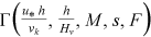in which is a function to be defined by the velocity measurements, ν_k is the water kinematic viscosity, M is the stem concentration which has to be considered as M/1 being 1 stems dm⁻² a reference concentration (Carollo et al., 2005), s is the energy slope, F =  is the flow Froude number, and δ is a coefficient which can be calculated by the following theoretical equation (Barenblatt, 1991; Castaing et al., 1990):

()

in which Re = V h/ν_k is the flow Reynolds number.

Considering that the ratio between u_*h/ν_k and h/H_v is equal to the shear Reynolds number Re_*, and F and Re_* are related (Baiamonte & Ferro, 1997; Ferro, 2018), Equation (2) can be rewritten as follows:

()

in which is a function to be defined by velocity measurements.

The velocity distribution (Equation 4) can be integrated, and the following expression of the Darcy–Weisbach friction factor f is deduced (Barenblatt, 1993; Ferro, 2017; Ferro & Porto, 2018a):

()

Setting into Equation (4) y = α h, being α h the distance from the bottom at which the local velocity is equal to the cross-section average velocity V, the following estimate Γ_v of Γ function (Ferro, 2017; Ferro & Porto, 2018a) is obtained:

()

The coefficient α < 1 takes into account that (i) a mean velocity profile in the cross-section is considered (i.e., the velocity profile is obtained by averaging for each distance y the velocity values v measured in different verticals, and its integration gives the cross-section average velocity), and (ii) the average velocity V is located below the water surface. Ferro (2017) proposed the following theoretical relationship to calculate the coefficient α:

()

According to Equation (4), Γ theoretically depends on the submergence ratio, the stem concentration, the channel slope, and flow Froude number (Ferro, 2018) and its estimated value, Γ_v, can be obtained by the following power equation (Ferro, 2019):

()

in which a, b, c, d, and e are coefficients to be determined from experimental measurements. The accuracy of Equation (8) depends on the accuracy of both the measured variables (s, F, h/H_v, and M) and the estimate of the listed coefficients. The numerousness of the available database affects this last estimate.

2.2 Experimental data

The available experimental measurements were carried out in a flume at the laboratory of the Department of Civil, Architectural, and Environmental Engineering of the University of Naples “Federico II” (Figure 1). The flume, having a variable slope (0.01–0.03), was 8 m long and had a rectangular cross-section 0.4 m wide and 0.4 m high. Rigid vegetation, arranged in the whole channel bed, was simulated by rigid cylinders with height H_v = 1.5 cm and a diameter of 0.4 cm. The experimental runs were carried out using two arrangements (staggered ST and aligned AL) and three different concentration values M (4, 8, and 16 stems dm⁻²). The measurements (60 experimental runs) were done for submergence ratio h/H_v ranging from 1.53 to 8.78, that is, for marginally inundated flow regime (1 ≤ h/H_v ≤ 2) and well-inundated flow regime (h/H_v > 2) according to Lawrence, (1997, 2000) (Carollo & Ferro, 2021). The investigated flows were turbulent (5467 ≤ Re ≤ 103,506) and were characterized by Froude numbers ranging from 0.51 to 1.7. Further details on the experimental tests are reported in the paper by Gualtieri et al. (2018). The characteristic data of the experimental runs (slope s, stem concentration M, Re, and F) are listed in Table 1.

Table 1. Characteristic data of the experimental runs by Gualtieri et al. (2018).

Arrangement	Run	slope s	Stem concentration M (stems dm−2)	Re	F	Coefficient of Equation (13) a
Staggered	B3	0.03	8	11,757–92,781	1.08–1.50	0.3376
	B5	0.02	8	12,005–67,979	0.94–1.23
	B6	0.01	8	10,279–76,532	0.70–0.94
	B8	0.03	4	25,954–103,506	1.49–1.70	0.3381
	B10	0.01	4	12,998–63,625	0.88–1.08
Aligned	B1	0.01	16	5467–103,051	0.53–0.88	0.3395
	B2	0.03	16	7507–103,189	0.88–1.37
	B4	0.01	8	9156–101,768	0.71–0.95	0.3397
	B7	0.03	4	16,997–95,458	1.40–1.69	0.3387
	B9	0.01	4	12,998–88,274	0.88–1.10

3 RESULTS

The measurements carried out in different arrangements (staggered ST and aligned AL) were first represented by the f − h/H_v plot (Figure 2). These measurements demonstrate that a strong relationship exists between the Darcy–Weisbach friction factor and the submergence ratio, and, for concentration values less than or equal to 8 stems dm⁻², the flow resistance law is not affected by the arrangement (staggered, aligned) of the vegetation elements.

Using the measurements (37 experimental runs) corresponding to the staggered arrangement with two concentration values M (4 and 8 stems dm⁻²) Equation (8) was calibrated:

()

which is characterized by a coefficient of determination equal to 0.9984. The coefficients of Equation (9) were estimated by a least-squares technique which uses the linearization of Equation (8).

The comparison between the measured values of Γ_v (Equation 6) and those calculated by Equation (9), distinguishing the pairs corresponding to different concentration and slope values, are plotted in Figure 3a. Coupling the theoretical expression of the Darcy–Weisbach friction factor (Equation 5) with Equation (9) allows for calculating f considering the effect of flow condition (F, h/H_v) and the characteristics of vegetation (arrangement and stem concentration). The friction factor values calculated by Equations (5) and (9) are characterized by a good agreement with the measured f values (Figure 3b) and errors in the estimate E are always less than or equal to ±2.5% and less than or equal to ±1.5% for 81.1% of the examined cases.

As Equation (9) suggested a limited effect of M on the estimate of Γ_v, the following equation was considered:

()

Using the measurements (37 experimental runs) corresponding to the staggered arrangement the values a = 0.3390, b = 1.0715, c = 0.5682, and d = 0.0396 were obtained. Equation (10), with the listed values of the coefficients a, b, c, and d, is characterized by a coefficient of determination equal to 0.9982. For the staggered arrangement, the agreement between the measured friction factor values and those calculated by Equation (5) coupled with Equation (10) is characterized by errors in the estimate E which are always less than or equal to ±2.5% and 78.4% of the errors are less than or equal to ±1.5%.

Using the measurements (40 experimental runs) corresponding to the aligned arrangement with three concentration values M (4, 8, and 16 stems dm⁻²), the coefficients a = 0.3371, b = 1.0708, c = 0.5687, and d = 0.0448 of Equation (10) were obtained. The comparison between the measured values of Γ_v (Equation 10) and those calculated by Equation (9), distinguishing the pairs corresponding to different concentration and slope values, are plotted in Figure 4a. For the aligned arrangement, the agreement between the measured friction factor values and those calculated by Equation (5) coupled with Equation (10), plotted in Figure 4b, is characterized by errors in the estimate E which are less than or equal to ±2.5% for 77.5% of the cases and 57.5% of the errors are less than or equal to ±1.5%.

Considering that the analysis of the friction factor measurements (Figure 2) demonstrated that flow resistance law is not affected by the arrangement (staggered, aligned) of the vegetation elements, and the exponents b, c, and d of Equation (10) of the two arrangements are similar, Equation (10) was calibrated using the whole database (77 experimental runs):

()

which is characterized by a coefficient of determination equal to 0.9979. Figure 5 shows the good agreement between the measured friction factor values and those calculated by Equation (5) coupled with Equation (11). Considering that Equation (11) establishes that the exponents b = 1.0687, c = 0.5678, and d = 0.0437 can be assumed independent of stem concentration and vegetation arrangement, Equation (8) can be rewritten as:

()

in which is a function of the stem concentration and .

For a given vegetation arrangement (staggered, aligned) and stem concentration, the corresponding experimental run was used to estimate the function , and the developed analysis demonstrated that Equation (12) has the following expression:

()

in which a is a coefficient, depending on vegetation element arrangement and stem concentration, whose values are listed in Table 1. Figure 6 shows, as an example for the staggered arrangement and M = 8 stems dm⁻², the agreement between the pairs (X, Γ) and Equation (13), while the a values listed in Table 1 demonstrate that this coefficient can be considered independent on stem concentration and equal to 0.3380. For the aligned arrangement, the low variability of the a values listed in Table 1 allows assuming an average value of 0.3393.

The frequency distribution of the errors in the estimate of the Darcy–Weisbach friction factor calculated by Equation (5) coupled with Equation (11) and with Equations (5) and (13) are plotted in Figure 7. This figure demonstrates that using Equations (11) or (13) for estimating Γ_v gives f values characterized by similar errors and always less than or equal to ±5% and less than or equal to ±2.5% for 88% of the investigated cases.

4 DISCUSSION

The comparison between the pairs (h/H_v, f) corresponding to different arrangements and the same stem concentration (M = 4 and 8 stems dm⁻² in Figure 2) demonstrates that, for the investigated stem concentration values, the flow resistance law is independent of the vegetation element arrangement. This result agrees with previous studies (Ferro, 2019), obtained for the same arrangements (staggered, aligned) and M values ranging from 1.8 to 32 stems dm⁻², which established that the flow resistance is not affected by the vegetation arrangement and increases with M. This result can be justified considering that when the stem concentration is low the vegetation elements are so distant that no wake interference mechanism occurs (a wake generated downstream a cylinder extinguishes before of encountering the subsequent cylinder in the stream direction) and the dissipation is only controlled by the stem concentration.

As Equation (9) shows that Γ_v decreases for increasing values of the stem concentration, the Darcy–Weisbach friction factor increases with M. This result, for the staggered arrangement and the concentration range 4–8 stems dm⁻², demonstrates that the investigated stem concentration is low and, as consequence, f increases monotonically with M (Figure 3b). In other words, the stem concentration is low and the quasiskimming flow regime (Carollo & Ferro, 2021; Carollo et al., 2005; Ferro, 2019), which corresponds to the invariance of flow resistance with M, is not yet reached. For the staggered arrangement, neglecting the effect of M on the estimate of Γ_v (Equation 10) does not affect the agreement between the measured friction factor values and those calculated by Equation (5) coupled with Equation (10). This effect is due to the low investigated values of concentration M and the limited range of M values explored for the staggered arrangement (Table 1).

For the aligned arrangement, Figure 4 demonstrates that, for increasing stem concentration values from 4 stems dm⁻² (B7 and B9 arrangement) to 8 stems dm⁻² (B4 arrangement) and 16 stems dm⁻² (B1 and B2 arrangement), the Darcy–Weisbach friction factor shows an increasing trend. The differences in f values corresponding to 4 and 8 stems dm⁻² are limited, while they become appreciable for the highest investigated stem concentration. This result can be justified considering that, for the aligned arrangement, the investigated stem concentration values are low, and the quasiskimming flow regime is not yet reached. Figure 5, which shows the comparison between the measured friction factor values and those calculated by Equation (5) coupled with Equation (11), confirms that the hydraulic behavior of the two investigated arrangements is very similar, and the flow resistance equation is able to reproduce this hydraulic condition. For the two investigated arrangements, the a values listed in Table 1 demonstrate that the theoretical flow resistance law is able to estimate comparable values of the Darcy–Weisbach friction factor values confirming that this result is due to a low M value. The flow resistance law is also able to estimate the greatest f values (Figure 5) which, were measured for the aligned arrangement with M = 16 stems dm⁻².

The frequency analysis of the errors (Figure 7) demonstrated that the theoretical flow resistance equation (Equation 5) coupled with Equation (11), or Equation (13) allows an accurate estimate of the Darcy–Weisbach friction factor, which is characterized by errors that are always less than ±5%. This result can be justified considering that the investigated stem concentrations are low and the effect on the friction factor estimate is limited.

5 CONCLUSIONS

In this paper, flume measurements collected by Gualtieri et al. (2018) were used to study the effect of rigid submerged vegetation on the estimate of flow resistance. The theoretical flow resistance equation was calibrated and tested by the available experimental runs carried out in a flume where rigid cylinders were set in two arrangements (staggered, aligned) at high submergence ratios (ratio between the water depth and the vegetation height greater than 5). In particular, the Γ function of the power velocity profile was empirically related to the channel slope, the flow Froude number, and the submergence ratio. This calibration was carried out by distinguishing measurements corresponding to different vegetation arrangements (staggered, aligned) (Equation 10), joining all available data (Equation 11), and using only a scale factor representing the effect of vegetation arrangements (Equation 13). The analysis demonstrated that the theoretical flow resistance equation coupled with Equations (11) or (13) allows an accurate estimate of the Darcy–Weisbach friction factor, which is characterized by errors that are always less than 5% and less than or equal to 2.5% for 88% of the investigated cases. The results of this research are limited by the investigated arrangements and the M values ranging from 4 to 16 stems dm⁻². Other experimental investigations should be developed using higher stem concentration values to detect the trend with M and starting point of a skimming flow regime.

ETHIC STATEMENT

None declared.