Estimation and analysis of vegetation parameters for the water cloud model
Abstract
The Water Cloud Model (WCM) plays a crucial role in active microwave soil moisture inversion applications. Empirical parameters are important factors affecting the accuracy of WCM simulation, but the current evaluation of empirical parameters only considers the forward simulation process, and insufficient consideration is given to the model inversion problem. This study proposes a new estimation method for vegetation parameters in the WCM by combining the soil backscattering model and the objective function. The effectiveness of the method is then verified using measured data. Simultaneously, this study also analyzes the factors influencing the evaluation of vegetation parameters in the WCM, resulting in the following conclusions. First, blindly utilizing vegetation parameters recommended by previous model studies is not advisable. To ensure the accuracy of the simulation, it is necessary to adjust the vegetation parameters appropriately. Second, to ensure the ability of the WCM solving both forward and inverse problems, it is advisable to consider both soil backscatter and surface backscatter simulations in the construction of the cost function. Third, soil backscatter simulations have an impact on the solution of vegetation parameters, and more accurate soil scattering models provide a better representation of the modeled vegetation. This study presents a dependable method for resolving the vegetation parameters of the WCM, thereby offering a valuable reference for the application of the model in surface parameter inversion research.
1 INTRODUCTION
Soil moisture, as a pivotal variable in surface water and energy cycles, holds a critical role in climate change (Berg & Sheffield, 2018; Douville & Chauvin, 2000), drought monitoring (Ma et al., 2022; Zhu et al., 2021), flood warning (Kim et al., 2018), and various other aspects of considerable significance. Currently, soil moisture estimation predominantly relies on passive microwave remote sensing inversion (Chaubell et al., 2020; Zhao et al., 2021). However, the spatial resolution of the inversion results remains low due to inherent limitations in remote sensing data. Consequently, there is a persistent absence of high-resolution soil moisture products. To address this issue, it is crucial to focus on active microwave remote sensing inversion research. The primary approach to tackle this problem lies in studying and developing available models. The Water Cloud Model (WCM) is a fundamental and widely employed semi-empirical model in active microwave soil moisture inversion (Bao et al., 2018; Kong et al., 2018; Li & Wang, 2018; Prevot et al., 1993a). Many models refer to this vegetation layer modeling method (Hoekman et al., 1982; Mo et al., 1982). Research on WCM not only offers an effective approach to developing high-resolution soil moisture products but also aids in expanding the application scope of active microwave remote sensing data in surface parameter inversion.
In the formula, represents the backscattering coefficient of the land surface. denotes the volume scattering of the vegetation canopy. corresponds to the backscattering coefficient of the soil. and are vegetation descriptor parameters, which is set as in this study. is vegetation water content, measured in kg/m2. represents the two-way transmittance of vegetation. θ denotes the incident angle. represents the volumetric moisture content of the soil measured in m3/m3. A, B, C, and D, are empirical parameters of the model.
Since the inception of the WCM, obtaining accurate empirical parameters has been a challenging task. This is primarily due to the difficulty in separately measuring the backscattered components of soil and vegetation. To address this issue, some studies have employed soil backscattering models as a substitute for Equation 4 to estimate the backscattering contribution of the soil. This approach helps to limit the interaction of vegetation parameters with soil parameters and to reduce the number of empirical parameters in the WCM. By substituting the estimated soil backscattering results into Equation 1, Bindlish and Barros (2001) carried out rate determinations of vegetation parameters for WCM on grass, wheat and pasture. Despite only focus on estimating vegetation parameters for a portion of the underlying surface, this study serves as the primary reference for subsequent research on parameter values in the application of the WCM (Jiang, 2020). Additionally, studies also focus on methods for solving the model parameters. These studies address the parameter estimation challenge by formulating it as a least squares optimization problem using the objective function method (Kumar et al., 2014; Li & Chen, 2020). As mentioned above, the WCM is a forward model, so surface backscatter is often the only simulated target used to construct the objective function and drive the iteration of parameters in most of studies. Parameter iteration focusing only on forward simulation could lead to parameter overfitting and deficiencies in the model's ability to solve inverse problems. After all, WCM are often used for inversion of surface parameters and their ability to solve inverse problems is crucial.
In summary, the empirical parameters of the WCM play a crucial role in determining the accuracy of model simulations. However, the current research on the values of these parameters remains vague and lacks consensus. Most of studies focus on the accuracy of the model parameters to carry out forward simulations, and there is a lack of consideration of the accuracy of the model to solve the inverse problem. In this study, we propose a method for assessing vegetation parameters that considers both forward and inverse simulation accuracy of WCM. The effectiveness of the method is verified based on measured data. It is hoped that this study can provide a powerful reference for the application of the WCM.
2 DATA
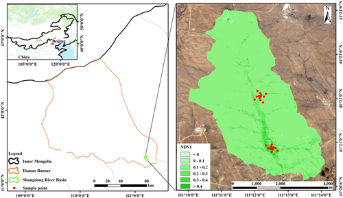
In this study, measured data collected from the Shangdong river basin are utilized to evaluate the vegetation parameters of the WCM. It is important to note that while the data used in this study are specific to the Shangdong river basin, the method employed for parameter estimation is not limited to this particular area. The following is a brief introduction to the data collection area and collection methods.
2.1 Study area
The Shangdong river basin is located in Baotou City, Inner Mongolia. The basin has a mid-temperate continental monsoon climate, with an average annual precipitation of 282.4 mm. The average altitude in the basin is 1602 m. The predominant soil types within the basin are sandy and light loam. The sandy soil is uniformly distributed across the entire watershed, while the presence of loam soil is primarily observed in areas with dense vegetation coverage within the catchment area of the watershed. The zonal vegetation within the basin comprises herbaceous plants that thrive under temperate semi-arid and arid climatic conditions. The plant community exhibits a straightforward structure, characterized by modest vegetation height and low moisture content. In terms of spatial distribution, vegetation is relatively densely distributed in the south-central part of the watershed and sparsely distributed in other areas.
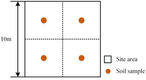
This study collected measured data from 23 monitoring sites in the basin, and each site represents a area. Measured data include soil moisture, vegetation moisture content, and surface roughness at the time of satellite transit. The locations of the measured points are shown in Figure 1.
2.2 Soil moisture data
In the given formula: is the volumetric moisture content of the soil; and are the dry density of the soil and the density of the water, measured in g/cm3, 1.45 and 1 is used in this study; and are the wet weight and the dry weight of the sampled soil, measured in grams.
2.3 Vegetation moisture data
In the formula: is the vegetation moisture weight per unit area, kg/m2; and are the wet weight and the dry weight of the sampled vegetation, measured in kilograms.
2.4 Land surface roughness
In the formula: is the surface roughness, measured in m; is the elevation of the i-th point in a certain 1 m sampling length, the unit is m; is the average of all elevations in a certain 1 m sampling length.
2.5 Sentinel-1 radar data
Sentinel-1 is an Earth observation binary system jointly developed by the European Commission and the European Space Agency. It comprises two satellites: Sentinel-1A and Sentinel-1B. Both of them are equipped with C-band synthetic aperture radar (SAR), operating at a frequency of 5.405 GHz. Notably, they have the capability to simultaneously receive dual-polarization backscatter information. The source data utilized in this study comprises the GRDH data obtained after multi-view processing by the Sentinel-1A satellite in Interferometric Wide working mode on May 21, 2021.
In the formula: is the backscattering coefficient; is the gray value of the electrical signal; is the absolute scaling coefficient; θ is the local incident angle of the radar image.
3 METHOD
In this study, the soil backscattering, simulated by the OH model, is substituted into the WCM to evaluate vegetation parameters. The evaluation method uses the objective function approach, which converts the parameter estimation problem into a least squares optimization problem. To preserve the fairness of the positive parameter solution, this study randomly divide the 23 monitoring points into six parts and randomly used five of them to construct the cost function for the iteration, using the remaining one part for validation.
3.1 Simulation of soil backscattering
In the formula: , are the backscattering coefficients of soil for VH and VV polarization respectively; represents the cross-polarization ratio; is the incident angle of the electromagnetic wave; is the wave number, the calculation formula is k = 2π/λ, λ is the wavelength of the electromagnetic wave; s is the surface roughness, measured in m.
3.2 Objective function construction
In the given mathematical expression, serves as the objective function. represents the backscattering coefficient in the VV polarization observed by the Sentinel satellite at the i-th monitoring point. represents the soil VV polarization backscattering calculated by the OH model at the i-th monitoring point. and are weight parameters, which are both set to 1 in this study because this study considers forward and reverse modeling to be equally important.
3.3 Parameter optimization algorithm
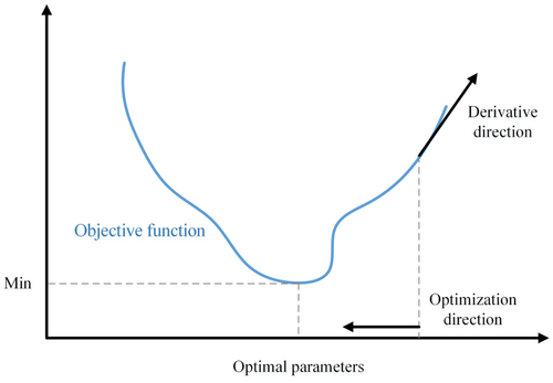
After the objective function is determined, solving the values of the A and B parameters when the objective function is minimized becomes the main task. This study employs the gradient descent algorithm (Haji & Abdulazeez, 2021) to optimize the values of parameters A and B. As a fundamental parameter optimization technique, the gradient descent algorithm plays a pivotal role in machine learning and optimization. Its core principle can be succinctly summarized as follows: the optimization direction for adjusting model parameters corresponds to the reverse direction of the derivative of the objective function with respect to those parameters, as illustrated in Figure 3. In contrast to alternative optimization algorithms, including Newton's method and the fastest gradient descent method, the primary advantage of this approach is its lack of reliance on second-order derivatives. This characteristic results in a lower threshold for application and broadens its applicability across various domains. However, it is important to acknowledge its limitations, which primarily manifest as suboptimal iteration efficiency and sluggish convergence speed. Despite these drawbacks, they do not preclude the utility of this method in the context of this study.
In the formula, and are the values of the A and B parameters in the m-th iteration respectively. represents the rate of change, which plays a crucial role in controlling the speed of convergence and is set to 0.05 in this study. and are the partial derivatives of the cost function with respect to the A and B parameters when and respectively.
4 RESLUT
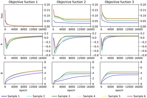
During this study's parameter optimization, the objective function decreases with more iterations. The changing trends of parameters A and B are shown in Figure 4. The figure illustrates a discernible trend of convergence between parameters A and B. Table 1 presents the results of the vegetation parameters, computed by the optimization algorithm for each respective objective function.
| Objective function | Polarization | A (Mean) | B (Mean) | Loss (Mean) |
|---|---|---|---|---|
| VV | 0.06928 | 4.742 | 0.002806 | |
| VV | 0.05562 | 3.659 | 0.05504 | |
| VV | 0.06464 | 3.840 | 0.06025 |
This study replaces the parameter calculation results into the WCM, computes the surface backscattering coefficient and soil backscattering coefficient for the remaining monitoring points, and employs the root mean square error as an evaluation index to assess the model's simulation accuracy. The final results are summarized in Table 2. It is evident that when the vegetation parameters recommended by previous studies are directly utilized, the simulation accuracy of the WCM decreases, whereas by employing the optimized vegetation parameters, the model's simulation accuracy has improved.
| RMSE | Reference values | |||
|---|---|---|---|---|
| Surface backscattering | 0.01156 | 0.01740 | 0.01591 | 0.06622 |
| Soil backscattering | 0.05581 | 0.05399 | 0.05266 | 0.06695 |
5 DISCUSSION
5.1 Iterative change analysis of vegetation parameters
During the parameter optimization process for the three objective functions, the trends in the parameters exhibit relative consistent. Specifically, the A parameters demonstrate an initial decrease followed by an increase, while the B parameters exhibit a consistent upward trend. This study attempts to analyze the reasons.
It can be seen from Equation 1 that there is a linear relationship between soil backscattering and surface backscattering. Given the reference parameter values (Bindlish & Barros, 2001), we compute the slope and intercept of the linear relationship using the measured data, and find that the slope is between 0.98 and 1 and the intercept is very close to 0. Remarkably, this linear relationship closely approximates the y = x function using reference parameter values. However, the analysis of the measured data fitting reveals that this linear relationship lies below the y = x function, as depicted in Figure 5. During the parameter optimization process, in an effort to promptly minimize the residual error in the simulation results, the linear function represented by the model undergoes an initial rapid downward translation. The intercept of the linear function decreases rapidly during this process, so the A parameter decreases rapidly during the initial iteration process. When the linear relationship moves down to a certain position, this overall downward translation will stop, and the reduction of the residual mainly depends on the reduction of the slope. Throughout this process, the decrease in slope results in a gradual increase in the intercept. Consequently, the A parameter exhibits a trend of initial decrease followed by an increase. And throughout this entire process, it is evident from the monotonic behavior of the exponential function that the parameter B consistently increases. This analysis further reveals that the parameters A and B predominantly depend on the statistical correlation between the soil backscattering coefficient and the surface backscattering coefficient.
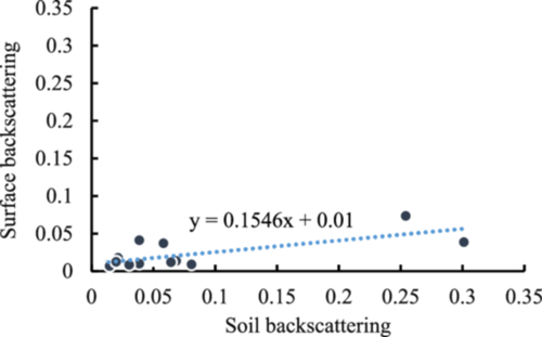
5.2 Objective function analysis
This study employs three distinct objective functions for the estimation of vegetation parameters. However, the outcomes of the parameter calculations exhibit some differences across these three objective functions.
Objective Function 1-2 primarily focuses on the simulation of surface backscattering and soil backscattering respectively. When contrasted with the initial values of the vegetation parameters, there has been a substantial enhancement in its simulation accuracy. This indicates that the parameter evaluation method in this study is effective. Comparing the parameter changes of objective functions 1 and 2, it is found that the direction and trend of parameter changes are more consistent, but the parameter convergence results are somewhat different. The former is caused by the measured data, while the latter is controlled by the objective function.
Comparison of the accuracy of the results for objective functions 1 and 2 reveals that both are more accurate on their respective simulated objects, but less accurate on non-simulated objects. This suggests that the model forward and inverse simulations do not require exactly the same model parameters. Considering only forward or inverse simulation of the model may result in overfitting of the model parameters. Overfitting in this context refers to the sacrifice of simulation accuracy in one direction of the model for the sake of improving simulation accuracy in the other direction. The design of the objective function 3 considers both the simulation accuracy of the WCM in forward and reverse directions. From the accuracy of the simulation results, the problem is well solved.
5.3 The meaning of parameters and the main factors affecting parameter evaluation
Analyzing the structure of the WCM, it's evident that the vegetation parameters primarily dictate the energy computations for both scattering and transmission within the vegetation layer. We first analyze the A parameter. As electromagnetic waves traverse the surface of the vegetation layer, their energy bifurcates into two distinct forms: absorption and transmission. The term in Equation 2 represents the fraction of energy that the vegetation layer absorbs. The product of the parameter A and the vegetation water content signifies the ratio of scattering energy to the energy absorbed by the vegetation layer. This is essentially the concept of the single scattering albedo. Hence, the parameter A serves as the conversion coefficient between the single scattering albedo and the vegetation water content. Secondly, we turn our attention to the parameter B. When the transmittance of vegetation is articulated as an exponential function, the absolute value of the exponent signifies the optical thickness of the vegetation layer. After removing the impact of the incident angle on the optical thickness, the product of the parameter B and the vegetation moisture content is the optical thickness in the vertical direction of the vegetation layer. Hence, the parameter B acts as the conversion coefficient between the vertical optical thickness of the vegetation layer and the vegetation's moisture content.
In summary, the “A” and “B” parameters are theoretically associated with the structure and type of the vegetation layer. However, in the context of this study, the model parameters that have been solved may lose their significance in this respect. The data for this study were gathered from desert steppes, so the vegetation water content in these areas is typically low, generally not exceeding 0.3 kg/m². In this scenario, the transmittance of the vegetation layer is relatively high, thereby rendering the impact of vegetation on surface backscattering quite minimal. So, the backscattering coefficients of the soil and surface should be similar. However, in this study, a substantial discrepancy between the two is observed. As mentioned in section 5.1 above, the correlation between soil backscatter and surface backscatter affects the assessment of vegetation parameters for the WCM. Therefore, the accuracy of soil backscatter modeling has a serious impact on the assessment of vegetation parameters. If the simulation of soil backscattering has a large error, meaningless iterations in the vegetation parameter iterations will occur to eliminate this error, resulting in the model vegetation parameters losing their meaning as conversion coefficients for vegetation optical thickness and single scattering albedo.
While this perspective requires further substantiation through actual soil backscattering measurement data, it also underscores the substantial influence that soil backscattering simulation exerts on the computation of vegetation parameters within the WCM. Undoubtedly, the physical interpretation of the vegetation parameters within the WCM can be elucidated more distinctly by employing a more precise soil backscattering model.
6 CONCLUSIONS
- 1.
When employing the WCM, the empirical vegetation parameters suggested by prior studies may not align with the actual measured data. To guarantee the model's simulation accuracy, it becomes necessary to suitably adjust the vegetation parameters of the model.
- 2.
To ensure the accuracy of the WCM in solving the forward inverse problem, it is more appropriate to construct the objective function with both soil and surface backscatter as the simulation objectives.
- 3.
The relationship between soil backscatter and surface backscatter affects the solution of vegetation parameters, and a more accurate soil scattering model would better illustrate the physical significance of vegetation parameters.
Indeed, it is our sincere hope that this study serves as a valuable reference for future applications of WCM.
ETHICS STATEMENT
None declared.
Open Research
DATA AVAILABILITY STATEMENT
The data that support the findings of this study are available from the corresponding author upon reasonable request.


