2.1 Target classification and scope

Despite assessing all regular targets (i.e., those starting by “T”), we still separated them into different difficulty categories to compare and rank the different methods. We considered the target classification as described in reference 13 provided by the Prediction Center (https://predictioncenter.org/).¹⁴ There, the different targets submitted are divided into evaluation units (or domains), each classified as “template-based easy” (TBM-Easy), “template-based hard” (TBM-Hard), “hybrid template-based/free modeling” (TBM/FM), or “free-modeling” (FM) targets, depending on whether good templates could be found in the PDB at the time of the experiment. Only individual evaluation units were considered for method ranking. These are referred to as “targets” for the remainder of the text. In addition, individual target difficulties were computed by taking the average of the coverage of the best structural template and the HHsearch probability of the match between the target and the best template.

2.2 Model scoring

2.2.1 CASP13—Inclusion of torsion angle deviations

Many metrics for the evaluation of model accuracy have been developed over the years, especially in the context of CASP, and a large number are computed and made available through the Prediction Center. In CASP13, Croll et al.¹⁵ adopted, and built on, the same overall ranking score used for TBM models in CASP12,¹⁶ which was based on five metrics: (1) GDT_HA, the high-accuracy version of the Global Distance Test (GDT), rewarding parts of the target that could be reproduced with high precision³; (2) lDDT, a local difference distance test that evaluates how well the all-atom distance map of the target is reproduced by the model¹⁷; (3) CADaa, which compares residues' contact surface areas¹⁸; (4) Sphere-Grinder (SG), a measure of local environment conservation¹⁹; and (5) ASE, the accuracy self-estimate measure that assesses how well the coordinate error estimates provided by the predictors in the model indeed predict the real positional deviations from the target.¹⁴

To these metrics, Croll et al. added three other terms to evaluate the geometric fitting of models: the (1) backbone and (2) side-chain deviation scores, which measure the local difference of torsion angles in the model relative to the target¹⁵; and (3) the MolProbity clashscore, which assesses the number of serious clashes in the model. The overall CASP13 ranking score combining all metrics was given by:

with z as the adjusted z score of the underlying metric over all models for a given target.¹⁵

2.2.2 CASP14—Inclusion of geometrical improvement

In CASP14, we implemented an additional novel metric that evaluates whether the backbone of a predicted model is geometrically better than the experimental structure of the target, an evaluation for which no metric is yet available. This metric comes from the observation that experimental structures submitted to CASP for use as targets are not only biologically but also qualitatively diverse; for example, some may not correspond to a final model and may require further refinement steps that will improve the geometry of their backbone (see the example in Figure S1). Thus, assuming that the target structure corresponds to the ground truth may lead to low scores for models that actually lack problems present in the unrefined target and are, thus, likely more accurate. In order to account for that, we developed DipDiff, which is based on the DipScore.²⁰

The DipScore is a distance geometry-based metric and a local protein backbone validation score that is used for guiding automated protein model building with ARP/wARP at medium-to-low resolution^{20, 21} and as a general protein backbone validation score,²² being also useful for the identification of geometrically strained residues of potentially functional importance.²⁰ Briefly, it is computed based on the all-to-all interatomic distances between the backbone Cɑ and O atoms of the residue to be analyzed and its two flanking neighbors, and evaluates the likelihood of the observed combination of interatomic distances to be correct based on what is found in high-quality, high-resolution structures from the PDB and those expected from a random sampling of atoms around a target Cɑ; the closer to one the DipScore is, the more likely that conformation is to be geometrically correct. It is computed using DipCheck,²⁰ distributed through the ARP/wARP and CCP4²³ software packages.

To compare the models to the target structure, we followed an approach similar to that of Croll et al.¹⁵ and, for each target, computed the per-residue DipScore differences to the target, so that a positive value corresponds to a residue that has a better geometrical environment in the model than in the target structure, and a negative value to the inverse, and took the average difference as the DipDiff score. In order to evaluate the usefulness of this metric for assessment, we compared it to the different metrics in the S_CASP13 scoring function and those available through the Prediction Center by computing the Pearson Correlation Coefficient between the different metrics.

For ranking, we updated the S_CASP13 scoring function, giving the same weight to DipDiff as to the other backbone geometry evaluating scores:

with z denoting the adjusted z score of the underlying metric over all models for a given target, computed accordingly to Croll et al.,¹⁵ that is, a set of initial Z-scores for a given metric was computed based on the mean and SD of all models under consideration, all models yielding a Z-score below −2 were then considered as outliers and the Z-scores recomputed using the mean and SD computed excluding them. At the end, negative Z-scores were set to zero in order to reduce the penalty on groups who tested novel methods. S_CASP14 and S_CASP13 ranking scores were computed for all models, for all targets, but only the first model submitted by each method (model 1) was considered for ranking. Individual sidechain quality was assessed based solely on the CASP13 geometric score.

2.3 Template selection and scoring

For targets classified as TBM-easy or TBM-hard, we also compared their putative templates with the submitted structure. For that, we used the pre-computed results from running HHsearch²⁴ against the PDB at the time of target submission, which is available through the Prediction Center. For each target, the top 10 X-ray crystallographic matches that covered at least 50% of the modeled target sequence with a probability of the match of at least 70% were collected. For each template, we computed (1) the GDT_HA, (2) the CASP13 backbone and (3) sidechain scores, and (4) the DipDiff. For that, models were first superimposed on the target structure using LGA³ to find residue correspondences. This was carried out using the same LGA parameters used by the Prediction Center for target-template structural alignment.

2.4 Method ranking

In CASP, it is common to rank methods based on the sum of the ranking scores of their models across all targets they submitted models to. However, such an approach directly weights for the number of targets for which a given method submitted a model, and favors those methods that systematically underperformed but may have modeled one target particularly well. We believe it is fairer to reward methods based on their consistent ability to accurately predict structures and, in CASP14, ranked methods in the high-accuracy category based on the median S_CASP14. Only the methods that submitted models for at least 10 targets were considered, and were ranked based on their first model (i.e., the model submitted as their predicted best model, model 1).

Methods were also classified into different categories based on the group type provided by the Prediction Center (human or server) and the keywords made available through their abstract, especially the “DeepL” (Deep Learning, DL) keyword, which states whether DL-based approaches were used.

2.5 Evaluation of model usefulness for MR

For targets solved via X-ray crystallography, we were able to assess the usefulness of the models as MR search models. To do this we employed AMPLE,²⁵ an MR pipeline designed to rationally truncate inaccurately predicted regions of ab initio models. Here, AMPLE's single model mode²⁶ was modified to make use of the local RMS error estimates usually present in the B-factor column of the submitted models. These RMS error estimates were squared and multiplied by 8π²/3 so that they could be interpreted as B-factors and thereby downweight predicted unreliable contributions from the model in MR.¹⁵ They were also used to guide AMPLE's progressive truncation process through which the predicted least reliable regions of the model were removed in ~5% increments. MR solutions were verified using phenix.get_cc_mtz_pdb²⁷ where a global map correlation coefficient (map CC) ≥0.25 was considered a solution. Given the relatively large computational overhead of MR, this assessment with AMPLE was limited to AF2 models. Full-length models were used for all the datasets except T1032, T1073, T1080 and T1091, where it was apparent that the crystallized structure was only a fragment of the full length target: in those cases the part of the model corresponding to the crystallized section was used.

2.6 Code and data availability

All these steps were implemented as Python scripts and more details, as well as dependencies (e.g., pdb-tools²⁸ for the handling of PDB files incompatible with some tools), can be found in the source code, which is available at https://github.com/JoanaMPereira/CASP14_high_accuracy. The computed data, as well as a script for the individual calculation of the DipDiff given two structures, is also available through the same link. The modifications made to AMPLE are now available through CCP4.²³

3.1 Backbone geometric quality and accuracy

Before proceeding to method/group ranking based on model accuracy according to different metrics, we first looked at the individual targets and how their backbone geometry compared to that of their models. For that, we developed and used the DipDiff metric, which corresponds to the average per-residue DipScore difference between a given model and its target structure. Subtracting the per-residue DipScore of a predicted model to its reference structure provides us with information regarding those regions that are geometrically better (or worse) in a given model. The average of those differences tells us whether (1) a model has all geometric issues resolved without the introduction of other major ones (positive DipDiff), (2) a model has either the same geometric issues found in the target or fixed them while introducing others (DipDiff around 0), or (3) the model has several severe geometric issues not found in the target (negative DipDiff).

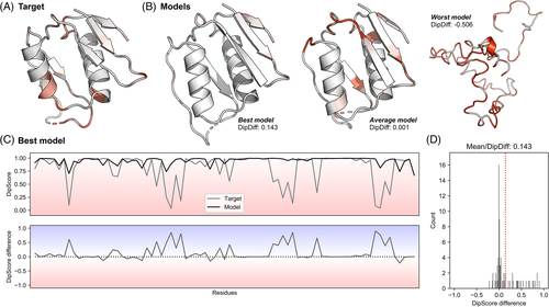
As an example, Figure 1A depicts the experimental structure of target T1047s2-D3, colored based on the DipScore of its individual residues (the redder, the lower the score). While most residues have a DipScore close to 1, at least 10 located mostly in loops and terminal helix regions are colored pink or red, indicating they have a very low DipScore and thus uncommon backbone geometries. One example is that of Asp344 (Figure S1), which has at least two stretched interatomic distances²⁰ not supported by the experimental electron density (Figure S1A). The observation that these two distances are shortened in the final (Figure S1B) deposited structure (PDB ID 7BGL), resulting in a favorable DipScore, supports the notion that the target structure was not a finalized, refined model. In Figure 1B, the structure of three models built for this target, selected to represent different model qualities, are shown and colored similarly. The first (best) model adopts the same overall fold as that of the target, but all geometrical problems seem to be absent. That is demonstrated by the per-residue DipScore distribution along the sequence (Figure 1C), with all residues in the target with a low DipScore having a score close to 1 in the model, translating into a positive DipScore difference in these regions. As the model lacks those severe geometric problems in the target without including others, its average DipScore difference (the DipDiff) is positive (Figure 1D). The second (average) model also corresponds to the same overall fold, but has a similar number of residues with an unlikely backbone geometry; these problems make the DipScore difference distribution wide while keeping the DipDiff close to 0 (Figure S2A). The third model, which is the worst model submitted for this target, does not fold as the target structure, but also most of its residues have a score close to 0, moving its DipDiff to extremely low values (Figure S2B).

The DipDiff is related to but does not correlate strongly with any of the scores included in S_CASP13 (Figure S3A); the closest is the CASP13 backbone geometry score, which measures the difference of backbone torsion angles in the model relative to the target, with a Pearson correlation coefficient of −0.54 (Figure 2B). Within all metrics pre-computed by the Prediction Center, DipDiff correlates the best with the MolProbity score (ρ = −0.53) and the percentage of Ramachandran favored and outlier residues (ρ = 0.74 and ρ = −0.68, respectively) (Figure S3B). This would be expected as all these metrics are also evaluators of overall protein backbone geometric quality. They, however, do not provide a comparison to the target and thus are not commonly used for the assessment of accuracy, which makes DipDiff a complement to the plethora of scores usually used in high-accuracy assessment.

Interesting to note is the relationship between DipDiff and GDT-HA, especially within CASP14. Although there is no linear correlation, there still exists a relationship between these two metrics (Figure 2A): a GDT_HA close to 100 always implies a DipDiff close to 0, but a lower GDT_HA may be accompanied by a variety of positive and negative DipDiff scores. Indeed, in a dataset where there is an equal distribution of target and model qualities, one should expect a “pyramid-shaped” relationship between DipDiff and GDT; the closer a model is to the target structure, the closest to the target is also its geometric quality. Exceptions would be those cases where all Cɑ are placed correctly but not the backbone oxygen atoms, for example, due to peptide flips. Such cases would have a perfect GDT but a very low DipDiff. However, such a “pyramid-behavior” is not observed for the models in CASP14, as 80% of the models have a negative DipDiff and 2% have a DipDiff above 0.1, especially at the 50–80 GDT_HA range.

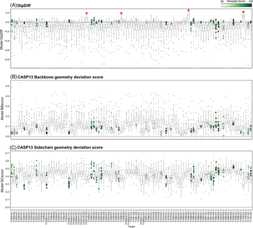
The distribution of DipDiffs across all targets (Figure 3A) demonstrates that indeed most are modeled with a mostly negative median DipDiff (the pan-target median of individual target median Dipdiff values in CASP14 is −0.06). Still, a few cases seem to have been systematically modeled with a better backbone geometry than the target itself (marked with a star in Figure 3A). These are T1047s2-D3 (median DipDiff 0.08), T1058-D1 (median DipDiff 0.05), T1085-D3 (median DipDiff 0.15) and T1100-D1 (median DipDiff 0.12, submitted by our group). By carrying out the same analysis for templates, it was interesting to observe that for most targets we found good templates with a positive DipDiff (Figure 3A), suggesting that: (1) even when a good template is available (even if only partial), methods may be ignoring this information to build their models or include biases to deviate from the template backbone geometry, building, in general, models with an unrealistic backbone geometry; and that (2) the same seems to be true when building a protein structure from experimental data.

3.2 Sidechain accuracy

When it comes to sidechain modeling, we used the score developed by Croll et al.¹⁵ in CASP13, which measures the difference of sidechain torsion angles in the model relative to the target. This metric varies between 0 and 1, and the closer to 0 the lower the deviation. Contrary to the backbone, where the median CASP13 backbone geometry deviation score was 0.1 (Figure 3B), side-chains seem to continue to be the hardest to predict correctly, with the median model side-chain geometry deviation score for each model between 0.4 and 0.5 (Figure 3C).

As expected from the relationship between side-chain and backbone geometry,^{29, 30} the closer the geometry of the models' backbone, the more accurate were the side-chain conformations predicted (Figure 2D). However, such a correlation is not observed between the sidechain geometry and the backbone geometric quality (Figure 2C): models may be predicted without backbone geometry problems but still have incorrect sidechain conformations, while accurate sidechains are always accompanied by a similar backbone geometric quality. When considering templates, on the other hand, the models submitted to CASP14 seem to outperform the geometry accuracy of the templates, independently on how close they are to the targets (Figures 2C,D and 3C).

3.3 Overall ranking

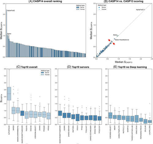
When we rank the different methods based on the median S_CASP14 of their first models, there is a clear leader, AF2, followed by three close runner-ups (Figure 4A), BAKER, BAKER-EXPERIMENTAL and Baker-RosettaServer (Figure 4A). AF2 has a median S_CASP14 of 2.2, which means the models it produces, and classifies as its best models, score in general 2.2 SDs better than the average model across all targets. In contrast, the three Baker methods have a median S_CASP14 of about 1.0 (BAKER 1.01, Baker-experimental 0.98, and the Baker-RosettaServer 0.86). When compared to the ranking obtained with S_CASP13, these four methods would rank the same way; the only difference lying in the places below, with S_CASP14 allowing for a better resolution in the lower places of the ranking (red arrows in Figure 4B).

Following these four methods, the accuracy of the next six methods is very similar, and here they would rank differently if the S_CASP13 scoring function were used. With S_CASP14 the ranking at these places is FEIG-R3 > FEIG-R2 > VOROCNN-SELECT > ZHANG > PROQ3D > PROQ2, while with S_CASP13 it would be PROQ3D > FEIG-R3 > VOROCNN-SELECT > ZHANG > FEIG-R2 > P3DE. The difference lies in the general geometric quality of the models these methods produce (Figure 5): while all these methods produce similarly accurate models based on the S_CASP13 metrics, the models generated by FEIG-R3, FEIG-R2 and VOROCNN-SELECT have a higher median DipDiff than those from PROQ3D and P3DE, which moves them higher in the ranking while pushing PROQ3D and P3DE down.

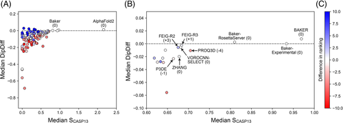
FEIG-R2 and -R3 are two methods from the same group that explore the structure prediction results from other servers to produce a model and further refine it using a molecular dynamics (MD) based method. FEIG-R2 uses the ZHANG/D-I-TASSER method and FEIG-R3 uses the Baker-RosettaServer, and while FEIG-R3 ranks below the Baker-RosettaServer due to deviations in the S_CASP13 metrics, FEIG-R2 ranks above ZHANG and ZHANG-SERVER/D-I-TASSER due to an increase in backbone geometric quality after refinement (Figure 5B). On the other hand, both VOROCNN-SELECT and PROQ3D use local model quality estimators for model ranking, but while PROQ3D uses a deep neural network trained in a variety of protein descriptor features and energy terms computed with Rosetta,³¹ VOROCNN-SELECT uses a combination of physics-based approaches and a deep convolutional neural network constructed on a Voronoi tessellation of protein structures,³² a rigorous way to define interatomic interactions, including local backbone geometric features.³³ The role of backbone geometric quality in ranking is even more drastic at the last positions, where non-accurate methods that produce models with a good backbone geometry are separated from those where not only does the model deviate drastically from the target but also its backbone has serious geometric problems (Figure 5A).

All top 10 ranking methods use deep learning-based approaches for modeling and/or ranking. The best non-DL-based method is VOROMQA-SELECT (Figure 4E), with a median S_CASP14 score of 0.66 (0.64 with S_CASP13 and a median model DipDiff of −0.02), ranking 13 overall. Contrary to VOROCNN-SELECT, this method from the same group uses a simple neural network (NN) trained to predict local (per-residue) CADaa scores from a Voronoi tessellation representation of the structure. MESHI is the second-best non-DL-based method and the first that does not use NN, ranking 26th in the overall ranking. This method uses a random forest regressor based on a set of sequence and structure features to estimate the GDT_TS of the model.

In the servers' section, the best method is Baker-RosettaServer, which is also the only server in the top 10 overall. Its leading position as the best fourth overall method makes it the most accurate method easily accessible to non-expert users. The following best servers are QUARK (14th), ZHANG-SERVER (D-I-TASSER, 17th), RAPTORX (30th), FEIG-S (32th) and TFOLD (33th), followed by variations of the ZHANG and TFOLD servers.

3.3.1 By target difficulty

We further assessed the accuracy of the different top 10 overall methods as a function of target difficulty, denoted by the four target categories defined by the Prediction Center (Figure 6). AF2 stands out as the most accurate across all target types, both at the overall level of the S_CASP14 score and its individual parameters (see the examples for median GDT_HA, median DipDiff, and median CASP13 geometry deviations score in Figure 6). It reaches a median GDT_HA around 80% at any level of difficulty, accompanied by a general slight improvement of the backbone geometry quality without large backbone geometry deviations from the target. Its sidechain modeling, however, is dependent on the target's category, but is always significantly better than any of the other methods (Figure 6E).

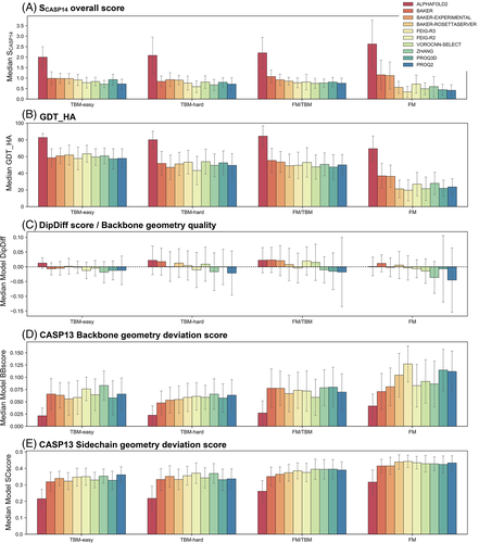
For the remaining methods, their ranking order varies depending on the target type, with this effect being more prominent for difficult, FM targets. In this category, both BAKER and BAKER-EXPERIMENTAL methods stand out from the other seven methods by achieving a median GDT_HA above 40% and a median S_CASP14 above 1.0, while the Baker-RosettaServer reaches a median GDT_HA of about 30% and a S_CASP14 below 1.0, comparable to that of the other five methods. Model backbone geometry quality is also dependent on the target difficulty for some methods, especially those in the lower half of the ranking (Figure 6C). Sidechains on the other hand seem to be as hard to predict for either target type, with most methods reaching a CASP13 sidechain deviation score around 0.4 in any category, although a slightly higher accuracy is reached for easy targets.

Unfortunately, AF did not participate in CASP14, which would provide a baseline for progress assessment. In order to circumvent that and evaluate the effect of target difficulty in the accuracy of the best model per target in CASP14 when compared to CASP13 and CASP12, we computed these metrics also for the CASP12 and CASP13 targets (using the data provided through the Prediction Center) and plotted them against the difficulty of all targets in the three CASP experiments (Figure S4). When compared to the effect of target difficulty in the accuracy of the best model per target, in CASP14 this dependency is eliminated due to the AF2 models, with the GDT_HA curve almost flat at around 80%, the CASP13 backbone deviation score below 0.05 and the CASP13 sidechain geometry score significantly below the CASP13 and CASP12 curves. When AF2 models are excluded, these curves approach the CASP13 behavior and values, but remain at better ranges, especially for GDT_HA and backbone geometry deviation scores. Most of these models were produced by BAKER methods, indicating that on average the BAKER methods reached accuracies higher than those of the best models in CASP13, produced by AF. This is, however, not the case for sidechain building and backbone geometry quality; for these metrics the best models in CASP14 excluding AF2 are as accurate as the best models in CASP12 and CASP13. Indeed, only AF2 brought an increase in sidechain accuracy since CASP12. Similarly, there is a tendency for improvement in model backbone geometry quality from CASP13 to CASP14, but this is not as significant as for the other metrics.

3.4 Model usefulness for MR

AMPLE's single model mode was used to assess the performance of AF2 models as search models in MR. Of the 32 datasets, we were able to solve 30 (94%). Twenty-six of these solutions required no truncation by AMPLE to succeed, although the majority (69%) gave better MR solutions (higher LLG, TFZ, map CC) with modest truncation. In some cases, the improvement was significant: for example, the map CC for the untruncated AF2 model for T1083 was 0.499, improving to 0.603 for the AMPLE version truncated to 69% of the original. Four targets only met our threshold for solution (map CC ≥0.25) after removing 15%–75% of the model with AMPLE (Figure 7): Where truncation levels are defined as the percentage of the original model retained after truncation, T1030 worked over a range of 18%–44% truncation levels, T1070 worked over a range of 19%–75% truncation levels, T1085 worked over a range of 21%–85% truncation levels and finally, T1100 worked over a range of 20%–25% truncation levels.

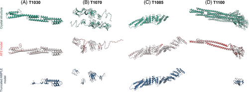
The AMPLE solutions for T1030 (Figure 7A), T1070 (Figure 7B) and T1100 (Figure 7D) represent cases where AF2 has accurately modeled a local region of the target protein but has not sufficiently captured the global shape for successful MR. In these examples, AMPLE's truncation process was able to automatically edit the original model down to a sufficiently accurate substructure that succeeded in MR. For T1085 (Figure 7C), the modeling overall gave a low GDT_HA (58.59), largely due to an additional domain in the model not present in the crystal structure. Looking at the 3 domains that aligned with the crystal structure, the GDT_HA scores were significantly higher (75.62, 84.75 & 75.88). While we would have expected this extra domain to have interfered with crystal packing, surreptitiously it extended into a solvent channel. Meanwhile, an extended ɑ-helix at the C-terminus of the structure was sited at an interface between proteins in the crystal lattice and did result in packing errors. Therefore, the removal of this ɑ-helix through modest truncation (85% of the original structure) by AMPLE was all that was required for MR to succeed.

Given the remarkable general success of AF2 models, it is of interest to examine the cases where they failed, even with truncation. T1032 is a hexameric structure at 3.3 Å resolution. The AF2 models trimmed to match the crystallized target were fairly close to the target (GDT_HA: 75.57, Figure 8A) but the moderate resolution and six molecules in the asymmetric unit make this target a challenge for MR. T1091 meanwhile is a dimeric structure composed of four domains linked by flexible loops. The trimmed AF2 models (Figure 8B) gave a relatively poor GDT_HA score overall (52.30), likely due to the flexibility of the interlinking loops. The GDT_HA values of the individual domains were significantly higher (D1 = 82.73, D2 = 82.71, D3 = 80.66, D4 = 90.18). Indeed, after performing a simple MR with Phaser³⁴ on each of the four domains, D1 (the largest of the four) provided a solution (map CC of 0.284).

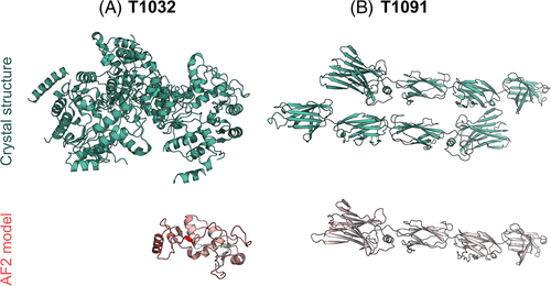
It can be seen therefore, that the AF2 models are close enough to the crystal structures to solve the majority of our datasets (31/32) with no modification (26), AMPLE truncation (4) or the use of individual domains (1). In the one case we were unable to solve, a decent AF2 model (GDT_HA: 75.57) was available but factors known to make MR difficult (resolution >3 Å, six molecules in the ASU) evidently hindered the solution. While this work was in review, similar findings have been reported elsewhere.³⁵