From digitized whole-slide histology images to biomarker discovery: A protocol for handcrafted feature analysis in brain cancer pathology
Xuanjun Lu, Yawen Ying and Jing Chen contributed equally to this work and shared the first authorship.
Abstract
Hematoxylin and eosin (H&E)-stained histopathological slides contain abundant information about cellular and tissue morphology and have been the cornerstone of tumor diagnosis for decades. In recent years, advancements in digital pathology have made whole-slide images (WSIs) widely applicable for diagnosis, prognosis, and prediction in brain cancer. However, there remains a lack of systematic tools and standardized protocols for using handcrafted features in brain cancer histological analysis. In this study, we present a protocol for handcrafted feature analysis in brain cancer pathology (PHBCP) to systematically extract, analyze, model, and visualize handcrafted features from WSIs. The protocol enabled the discovery of biomarkers from WSIs through a series of well-defined steps. The PHBCP comprises seven main steps: (1) problem definition, (2) data quality control, (3) image preprocessing, (4) feature extraction, (5) feature filtering, (6) modeling, and (7) performance analysis. As an exemplary application, we collected pathological data of 589 patients from two cohorts and applied the PHBCP to predict the 2-year survival of glioblastoma multiforme (GBM) patients. Among the 72 models combining nine feature selection methods and eight machine learning classifiers, the optimal model combination achieved discriminative performance with an average area under the curve (AUC) of 0.615 over 100 iterations under five-fold cross-validation. In the external validation cohort, the optimal model combination achieved a generalization performance with an AUC of 0.594. We provide an open-source code repository (GitHub website: https://github.com/XuanjunLu/PHBCP) to facilitate effective collaboration between medical and technical experts, thereby advancing the field of computational pathology in brain cancer.
Key points
What is already known about this topic?
-
Hematoxylin and eosin (H&E)-stained whole-slide images (WSIs) contain abundant information about cellular and tissue morphology. However, there remains a lack of systematic tools and standardized protocols for using handcrafted features in brain cancer histological analysis.
What does this study add?
-
This study presents a protocol for handcrafted feature analysis in brain cancer pathology to systematically extract, analyze, model, and visualize handcrafted features from WSIs, thereby promoting efficient collaboration between medical and technical experts.
1 INTRODUCTION
Histopathological slides, recognized as the “gold standard” for tumor diagnosis,1 hold significant value not only in the morphological assessment of diseases but also in critical biomedical information such as tumor heterogeneity, microenvironment characteristics, and molecular phenotypes.2 In the diagnosis and treatment of brain cancer, histopathological analysis using hematoxylin and eosin (H&E)-stained slides provides indispensable diagnostic evidence for clinical decision-making. However, the traditional diagnostic workflow relies on pathologists' visual inspection of slides under a microscope from low to high magnification. This qualitative analytical approach has inherent limitations. First, subjective interpretation is prone to variability because of differences in experience, leading to diagnostic inconsistency.3 Second, conventional examination has difficulty in quantitatively extracting subvisual tissue features, which may include crucial prognostic information.4 Third, the efficiency bottleneck of manual analysis becomes apparent when dealing with large numbers of slides.5 Thus, an accurate, objective, and interpretable protocol is an important goal in brain cancer pathology.
In recent years, the development of digitized whole-slide image (WSI) technology has revolutionized the field of pathology by enabling permanent digital storage of histopathological slides.6 Leveraging WSI, handcrafted features—i.e., features extracted by manually designed algorithms guided by domain-specific prior knowledge and empirical expertise—have been employed to extract attributes for the discovery of biomarkers. These features can derive quantitative prognostic, predictive, and other pathological information from H&E-stained WSIs, potentially transforming precision oncology and improving patient outcomes. Over the past few years, biomarkers based on handcrafted features have been extensively applied in numerous cancers, including head and neck squamous cell carcinoma,7 urothelial cancer,8 papillary thyroid carcinoma,9 hepatocellular carcinoma,10, 11 lung cancer,12, 13 oropharyngeal squamous cell carcinoma,14 and colorectal cancer.15 However, their application in brain cancer remains insufficient and is scarcely reported in the literature.
Current brain cancer research mainly focuses on radiology images,16-19 with few studies dedicated to histopathological analysis. Even within the limited pathological investigations, deep learning approaches dominate,20 yet their “black-box” nature results in a lack of interpretability, significantly hindering broader clinical translation. The substantial computational resource requirements and intricate preprocessing pipelines associated with deep-learning models pose additional barriers, further limiting their accessibility and practical adoption in clinical settings.
In this study, we present a protocol for handcrafted feature analysis in brain cancer pathology (PHBCP) based on H&E-stained WSIs. The protocol represents a simple, flexible, and modular open-source pipeline. We demonstrate the use of the protocol using two cohorts of glioblastoma multiforme (GBM). By following this protocol, medical and technical experts will be able to promote communication and collaboration, develop novel biomarkers, and collectively tackle clinical challenges in brain cancer, ultimately improving patient outcomes.
2 METHODS
2.1 Overview of the protocol
The protocol comprises seven main steps (Figure 1): (1) problem definition, (2) data quality control, (3) image preprocessing, (4) feature extraction, (5) feature filtering, (6) modeling, and (7) performance analysis. The problem-definition step specifies the precise clinical objectives to be analyzed. The data quality-control step aims to eliminate slides that contain contamination, artifacts, and other issues. The image-preprocessing step provides a WSI-based standardized preprocessing process, encompassing the region of interest (ROI) acquisition, WSI slicing, and color normalization. The feature-extraction step details the types, roles, extraction, and aggregation approaches for handcrafted features. The feature-filtering step refines a large set of redundant features to identify those most relevant to the label. The modeling step involves constructing models based on the filtered features to achieve optimal analytical performance. Lastly, the performance-analysis step visualizes important features and conducts downstream analyses. In this study, we use H&E-stained WSIs from two independent cohorts [The Cancer Genome Atlas (TCGA) and The Cancer Imaging Archive (TCIA)]21 to demonstrate how to use the PHBCP. The uniqueness of the protocol lies in its use of interpretable handcrafted features, rather than deep learning, to establish the complex relationship between WSI and the clinical question. Subsequently, Sections 3.2-3.8 correspond to steps 1–7, respectively.
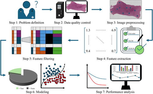
2.2 Problem definition
First, the clinical problem is determined, followed by the collection of tissue samples and corresponding pathology reports from patients. Slicing and staining operations were performed on the tissue samples. Stained tissue slides are converted into digital whole-slide histology images using digital scanners for subsequent computational pathology analysis. For example, one may want to interrogate the relationship between the nuclear shape features and the grade of tumor of the central nervous system.
2.3 Data quality control
The collected WSIs may be scanned by diverse clinical personnel utilizing different scanners across multiple institutions, which inevitably results in heterogeneous image quality. To mitigate the potential influence of these external variables on the experimental results, it is necessary to exclude substandard slides. However, the manual inspection of image quality in a high-throughput experimental context is often unfeasible. Consequently, a tool referred to as HistoQC22 is usually employed as an objective and rapid quality control process, identifying and flagging issues such as reagent contamination, artifacts, tissue folding, and staining irregularities, thereby enabling automated assessment of WSI quality. Combined with a pathological image viewer-QuPath,23 substandard data are excluded. Multicenter batch effects, such as stain variations, which may affect the robustness of the model. It is recommended to use Batch Effect Explorer24 to unveil the batch effect between cohorts.
2.4 Image preprocessing
In Section 2.3, we create a tissue mask, which excludes artifacts, tissue folding, and other external influences. In this step, the ROI of the current task is extracted from the tissue mask and split into image tiles of the desired size and magnification, for example, 224 × 224 pixels at 20x magnification, using the OpenSlide library,25 which is a Python library used for processing WSIs. To ensure a relatively dense tissue distribution, only those image tiles containing more than a certain proportion of tissue area are selected, for example, with 80% tissue area. To reduce computational load and avoid subjective selection bias, K-means clustering is performed on the tiles of each WSI to group tiles with similar phenotypes together. To ensure no critical regions are missed, E tiles are selected from each cluster, resulting in L × E tiles being used to characterize each patient, in which L is the number of clusters. Due to staining variations across different centers, deconvolution-based color normalization26-28 is applied to the selected tiles to eliminate color discrepancies between WSIs.
2.5 Feature extraction
Feature extraction refers to the process of transforming images into quantitatively described feature values. Five types of handcrafted features are provided in this protocol: first-order statistics (n = 17), gray level co-occurrence matrix (GLCM) features (n = 24), gray level run length matrix (GLRLM) features (n = 16), nuclear shape features (n = 25), and nuclear texture features (n = 13). First-order statistics describe the distribution of pixel intensity values within the tissue region. The GLCM features characterize the frequency of pairs of identical pixel intensity values in the tissue region. The GLRLM features describe the continuity of pixel intensity values over a specified distance in the tissue region. The nuclear shape features are employed to quantify the geometric properties of nuclear contours, thereby reflecting the characteristic patterns of nuclear deformation and cellular morphological changes during tumor progression. The nuclear texture features, by quantifying the heterogeneity and spatial configuration of chromatin distribution within the nucleus, enable an in-depth analysis of the structural distortions in the intranuclear microenvironment during tumor evolution. In total, 95 features can be extracted for each image tile. The details of the five types of features are as follows:
The other features, including entropy, energy, correlation, informational measure of correlation 1, and informational measure of correlation 2, are derived from GLCM features. Note that there are other types of handcrafted features, such as the spatial interaction between histological primitives,32, 33 that can be integrated into the PHBCP.
In summary, for each WSI, a feature matrix of size (L × E) × N can be obtained, in which N is the total number of extracted features. Based on this, users can aggregate and concatenate features using various methods according to their needs, for example, mean, standard deviation, and skewness.
2.6 Feature filtering
Feature filtering is a critical step in machine learning that identifies the most relevant and informative features from the feature matrix while eliminating redundant and irrelevant features. This process not only reduces the dimensionality of features but also mitigates overfitting, enhances model interpretability, and improves computational efficiency. In this study, the protocol employs comprehensive feature-selection methods to ensure robust and reliable features.
Firstly, to address multicollinearity and reduce feature redundancy, the PHBCP calculates the pairwise Spearman's rank correlation coefficient matrix among all features. Features with a correlation coefficient greater than the threshold, for example, 0.9 is generally used for removing features having more than 90% synchronicity, are removed. Subsequently, the feature matrix is standardized using the Z-score method.34 The above steps ensure that only non-redundant features are retained for further analysis.
Secondly, the protocol uses comprehensive feature selection methods to capture diverse aspects of feature importance and interactions. These methods include Lasso regression (LR), random forest (RF), elastic-net (EN), recursive feature elimination (RFE), univariate analysis (UA), minimum redundancy maximum relevance (MRMR), t-test, Wilcoxon rank-sum test (WRST), and mutual information (MI) methods, which are implemented in Python using scikit-learn, mrmr_selection, and scipy libraries. Here, users can select an appropriate number of features based on the sample size to achieve a suitable predictive performance and avoid overfitting and the curse of dimensionality.
Finally, each feature selection method is integrated with a classifier, and multi-fold cross-validation with user-defined iterations is performed to assess the consistency and reliability of the selected features across multiple data splits.
By combining correlation-based filtering with comprehensive feature selection methods and cross-validation, the protocol provides a robust framework to identify the most discriminative features while minimizing redundancy and overfitting.
2.7 Modeling
In this step, the PHBCP combines the feature selection methods and classifiers one by one to construct potential models. The protocol employs eight machine learning classifiers, including quadratic discriminant analysis (QDA), linear discriminant analysis (LDA), RF, K-nearest neighbors (KNN), linear support vector machine (LSVM), Gaussian naive bayes (GNB), stochastic gradient descent (SGD), and adaptive boosting (AdaBoost), which are implemented in Python using scikit-learn library. The eight classifiers are implemented in conjunction with the top features selected using the nine feature selection methods. The classifiers are evaluated with multi-fold cross-validation with user-defined iterations within a training cohort. Ultimately, the PHBCP identifies the optimal model combination from the 72 different combinations based on the highest average area under the curve (AUC) across user-defined iterations.
2.8 Performance analysis
Based on the optimal model combination determined during the modeling phase, one can conduct performance analysis focusing on the visualization of the top features' feature distribution, feature importance, and survival analysis in the external validation cohort.
Firstly, the PHBCP calculates the mean, median, and skewness of the top feature values, and then divides the feature values into equal bins to obtain 10 intervals. The distribution of the top features is visualized using histograms overlaid with kernel density estimation (Gaussian kernel) curves. Secondly, a horizontal bar is used to visualize the selection frequency percentage of the top features across the multi-fold cross-validation with user-defined iterations, highlighting the most important features and understanding their contributions to the optimal model combination. A higher selection frequency indicates a greater predictive contribution to the model and a stronger clinical relevance to the research question. Finally, the PHBCP locks down the optimal model combination and corresponding top features in the training cohort and conducts survival analysis in the external validation cohort. A Kaplan–Meier curve is used to evaluate, for example, the survival probability between predicted long- and short-term survival patients. The log-rank test was employed to examine survival differences, indicating the prognostic significance of the categorical variable on the survival endpoint. All tests are two-sided, with the significance level set at 0.05.
3 RESULTS
Given that GBM is the most common and aggressive type of malignant primary brain tumor,35, 36 we used a GBM survival prediction problem as an exemplary task to demonstrate how to use the PHBCP. First, WSI data and corresponding basic clinical information were obtained from two independent cohorts through The Cancer Genome Atlas (TCGA) (389 cases) and The Cancer Imaging Archive (TCIA, 200 cases).21 Subsequently, the entire tissue region was defined as the ROI, with overall survival (OS) established as the endpoint. For patients whose death occurred during the follow-up period, OS of less than or equal to 2 years was classified as short-term survival, while OS greater than 2 years was classified as long-term survival. For censored patients, the final follow-up time was used as the OS, with cases whose OS exceeded 2 years classified as long-term survival, while cases with an OS of less than or equal to 2 years were considered missing information and excluded from the analysis. OS was defined as the time from surgery to death.
In Section 2.3, HistoQC was used to exclude WSIs with fewer than 250,000 usable pixels as well as those exhibiting significant issues such as extensive blurring, tissue folding, reagent contamination, and abnormal staining. The detailed settings are provided in the supplementary parameter settings for HistoQC. For patients with multiple slides, one slide was selected for subsequent analysis based on its image quality using the pathological image viewer-QuPath. Inclusion and exclusion criteria were applied to both cohorts. Inclusion criteria: (1) patients who underwent resection and were confirmed to have GBM through surgical pathological specimens; (2) patients whose OS information was complete; (3) patients who contained follow-up information. Exclusion criteria: (1) missing H&E-stained WSIs of 20x magnification and (2) histopathological slides that did not meet the standard requirements for analysis. Ultimately, 207 patients from TCGA were included as the training cohort, while 57 patients from TCIA were incorporated as the external validation cohort. Table 1 presents a summary of the basic clinical information and distribution differences between the training cohort and the external validation cohort.
| Training cohort (N = 207) | External validation cohort (N = 57) | p | |
|---|---|---|---|
| Age | 0.8546 | ||
| ≤ 65 | 150 (72.5%) | 42 (73.7%) | |
| > 65 | 57 (27.5%) | 15 (26.3%) | |
| Sex | 0.9723 | ||
| Male | 124 (59.9%) | 34 (59.6%) | |
| Female | 83 (40.1%) | 23 (40.4%) | |
| Race | <0.0001 | ||
| White | 189 (91.3%) | 24 (42.1%) | |
| Asian | 3 (1.4%) | 19 (33.3%) | |
| Other | 11 (5.3%) | 13 (22.8%) | |
| Unknown | 4 (1.9%) | 1 (1.8%) | |
| History of LGG | |||
| Yes | 3 (1.4%) | NA | |
| No | 204 (98.6%) | NA | |
| Event status | 0.4987 | ||
| Occurred | 191 (92.3%) | 51 (89.5%) | |
| Censored | 16 (7.7%) | 6 (10.5%) | |
| Survival status | 0.5731 | ||
| Long term (>2 years) | 54 (26.1%) | 17 (29.8%) | |
| Short term (≤2 years) | 153 (73.9%) | 40 (70.2%) | |
- The p-values were calculated by Pearson's Chi-square test.
In Section 2.4, the tissue mask generated through HistoQC was aligned with the corresponding WSI, and image tiles of 224 × 224 pixels were extracted at 20x magnification without overlap. The tiles from each WSI were clustered into 10 classes, and 50 tiles were randomly selected from each class to ensure a comprehensive analysis of all regions. Stain normalization was performed on 500 selected tiles for subsequent feature extraction.
In Section 2.5, three types of features were extracted: First-order statistics, GLCM features, and GLRLM features, totaling 57 features. For each WSI, a feature matrix of size 500 × 57 was obtained, and the feature matrix was averaged to aggregate a 1 × 57 feature vector.
In Sections 2.6 and 2.7, in order to avoid the curse of dimensionality and overfitting, we set the number of top features to six, based on the experimental experience that the number of selected features should be approximately one-10th of the number of minority class samples. In this study, the training cohort contained 54 minority class samples and thus the top six features were chosen. The Spearman correlation threshold was set to 0.9. The predictive performance of the model in the training cohort was evaluated by performing 100 iterations of five-fold cross-validation in 72 model combinations to avoid incidental results. The detailed results are presented in Table 2. Table 2 shows that the optimal model combination was MI-KNN (AUC = 0.615 ± 0.027). The results for accuracy and F1 score are presented in Tables S1 and S2, respectively.
| QDA | LDA | RF | KNN | LSVM | GNB | SGD | AdaBoost | |
|---|---|---|---|---|---|---|---|---|
| LR | 0.595 ± 0.022 | 0.550 ± 0.029 | 0.597 ± 0.037 | 0.591 ± 0.028 | 0.511 ± 0.034 | 0.601 ± 0.028 | 0.533 ± 0.038 | 0.610 ± 0.033 |
| RF | 0.593 ± 0.028 | 0.564 ± 0.025 | 0.586 ± 0.033 | 0.580 ± 0.029 | 0.521 ± 0.039 | 0.582 ± 0.030 | 0.536 ± 0.046 | 0.578 ± 0.032 |
| EN | 0.572 ± 0.029 | 0.547 ± 0.021 | 0.598 ± 0.038 | 0.579 ± 0.032 | 0.527 ± 0.034 | 0.567 ± 0.027 | 0.532 ± 0.038 | 0.584 ± 0.035 |
| RFE | 0.585 ± 0.032 | 0.509 ± 0.032 | 0.577 ± 0.036 | 0.583 ± 0.039 | 0.454 ± 0.034 | 0.575 ± 0.022 | 0.513 ± 0.040 | 0.572 ± 0.034 |
| UA | 0.576 ± 0.028 | 0.565 ± 0.023 | 0.577 ± 0.034 | 0.557 ± 0.033 | 0.530 ± 0.032 | 0.553 ± 0.028 | 0.541 ± 0.040 | 0.590 ± 0.033 |
| MRMR | 0.573 ± 0.027 | 0.566 ± 0.022 | 0.586 ± 0.032 | 0.558 ± 0.033 | 0.540 ± 0.031 | 0.554 ± 0.026 | 0.545 ± 0.034 | 0.595 ± 0.040 |
| t-test | 0.572 ± 0.032 | 0.568 ± 0.020 | 0.579 ± 0.035 | 0.562 ± 0.030 | 0.537 ± 0.029 | 0.555 ± 0.024 | 0.535 ± 0.038 | 0.594 ± 0.035 |
| WRST | 0.596 ± 0.031 | 0.577 ± 0.025 | 0.588 ± 0.041 | 0.574 ± 0.036 | 0.532 ± 0.038 | 0.587 ± 0.028 | 0.548 ± 0.036 | 0.605 ± 0.034 |
| MI | 0.594 ± 0.025 | 0.528 ± 0.032 | 0.567 ± 0.039 | 0.615 ± 0.027 | 0.467 ± 0.036 | 0.591 ± 0.024 | 0.531 ± 0.041 | 0.586 ± 0.037 |
- Note: The bold values represent the AUC and standard deviation of the optimal model combination.
The top six features and their distribution from the MI-KNN model combination in Section 2.8 are illustrated in Figure 2. Six features closely approximated a normal distribution. The normal distribution indicates that these features were relatively stable within the patients, reflecting limited interindividual variability. The features shown in Figure 3 were used to analyze the contribution of the top 12 selected features to the MI-KNN model combination. The top two features, glcm_Contrast_average_20 and glcm_Imc1_average_20, were considered the most relevant to patient outcomes because of their highest selection frequency, underscoring their potential as biomarkers for GBM survival prediction. Finally, in the survival analysis of the external validation cohort, long-term survival patients showed higher survival probabilities compared with short-term survival patients, with statistically significant differences between the two groups (Figure 4), indicating that the constructed classification model had significant predictive value for survival endpoints in GBM patients. Based on the top six features of the MI-KNN model combination in the training cohort, a KNN classifier was trained. In the external validation cohort, the classification performance was observed with an AUC of 0.594, an ACC of 0.754, and an F1 score of 0.848.
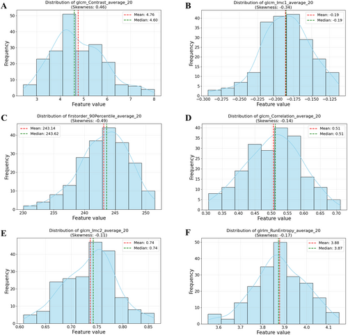
The distribution of the top six feature values in the training cohort (A–F) approximate a normal distribution. The x-axis represents the binned feature intervals (10 bins), and the y-axis indicates the frequency of samples.
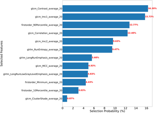
The top 12 features at selection frequency and their percentage contributions to the MI-KNN model combination across 100 iterations of five-fold cross-validation.
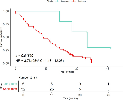
The Kaplan–Meier curve of GBM patients from the external validation cohort was stratified by the MI-KNN model combination into long-term and short-term survival groups.
4 DISCUSSION
In this paper, we develop and present a PHBCP. The presented protocol, termed PHBCP, offers a systematic, modular, and open-source framework and provides WSI processing and analysis guidelines in brain cancer. The results and methodology outlined in this protocol demonstrate its potential to enhance the discriminability and efficiency of brain cancer prediction and prognosis.
Features can be primarily categorized into two types: handcrafted features and deep learning-derived features. Handcrafted features are those extracted through manually designed algorithms, typically based on domain-specific knowledge or experience, such as texture features, statistical features, and geometric features.32 Given an input, these features yield a fixed and interpretable output. In contrast, deep learning-derived features are primarily learned automatically from data by deep learning models, without the need for manual design. Examples include features extracted by ResNet,37 CONCH38 and UNI.39 In practical application, models based on handcrafted features can provide interpretable and clinically relevant insights, which are essential for building trust among medical and technical experts. In contrast, although deep learning models have shown excellent performance in many tasks, these models typically rely on large amounts of data and cannot extract discriminative features from small samples. Additionally, the internal feature representations of deep learning models are complex, their decision-making processes are opaque, and it is difficult to explain their reasoning logic, resulting in poor interpretability. It is also challenging to incorporate specific medical prior knowledge into these deep learning models. These issues limit the widespread application of deep learning-derived features in clinical practice and, to some extent, hinder efficient collaboration between medical and technical experts. In this paper, PHBCP indicates the importance of these features in discovering novel biomarkers and improving the understanding of tumor heterogeneity, a key challenge in brain cancer research.
In the exemplary task of predicting 2-year survival in GBM, four of the top six features were related to GLCM, one feature was associated with first-order statistics, and one feature was connected to GLRLM. The glcm_Contrast_average_20 feature was identified as the most prognostically relevant image feature because of its highest selection frequency. This feature is utilized to quantify the local intensity variation. Through analysis, it was observed that the magnitude of contrast is often closely correlated with the area and distribution of tumors and necrotic regions. This correlation can be used to explain the reasoning logic behind survival prediction using image features. When combined with multiomics data, the biological significance underlying these images can be further elucidated.
By providing a step-by-step guide, the protocol enables seamless collaboration between medical and technical experts, fostering the development of innovative solutions to clinical problems. In this paper, the 2-year survival prediction in GBM serves merely as an exemplary task. Researchers can also conduct other brain cancer-related analyses based on PHBCP, such as isocitrate dehydrogenase (IDH) mutation analysis. The open-source nature of the protocol ensures its accessibility to a wide range of researchers, promoting reproducibility and scalability across different institutions and datasets.
The protocol has limitations. Although we have established a protocol for handcrafted features in brain cancer pathology, it does not encompass all types of handcrafted features. However, other researchers can add comprehensive handcrafted features to the PHBCP. As new pathological insights emerge, the reliance on handcrafted features may require continuous refinement. We anticipate that future contributions from medical and technical experts will enhance and expand this protocol.
5 CONCLUSION
The protocol presented in this study is a significant step forward in the analysis of handcrafted features for brain cancer pathology. By providing a structured and collaborative framework, it empowers pathologists and clinicians to harness histopathological data for improved brain cancer care. We anticipate that this protocol will serve as a valuable resource for the scientific community, driving innovation and promoting the diagnosis and treatment of brain cancer.
AUTHOR CONTRIBUTIONS
Xuanjun Lu: Methodology; data curation; validation; writing—original draft; software; investigation; formal analysis; visualization; funding acquisition. Yawen Ying: Methodology. Jing Chen: Data curation. Zhiyang Chen: Data curation. Yuxin Wu: Software; methodology. Prateek Prasanna: Data curation. Xin Chen: Resources; writing—review and editing. Mingli Jing: Writing—review and editing; resources. Zaiyi Liu: Writing—review and editing; resources. Cheng Lu: Conceptualization; methodology; project administration; funding acquisition; writing—review and editing; resources; software; writing—original draft.
ACKNOWLEDGMENTS
This study was supported by National Natural Science Foundation of China (82272084), National Key R&D Program of China (2023YFC3402800), Guangdong Provincial Key Laboratory of Artificial Intelligence in Medical Image Analysis and Application (2022B1212010011), and Postgraduate Innovation and Practical Ability Training Program of Xi'an Shiyou University (YCS23114144). The authors would like to thank the support provided by MediAI Hub, an advanced medical image analysis software developed and maintained by MediaLab. TCIA data used in this publication were generated by the National Cancer Institute Clinical Proteomic Tumor Analysis Consortium.
CONFLICT OF INTEREST STATEMENT
The authors declare no conflicts of interest.
ETHICS STATEMENT
Image and data of TCGA and TCIA are publicly available,21 and do not require ethics approval.
Open Research
DATA AVAILABILITY STATEMENT
Image and data of The Cancer Genome Atlas (TCGA) are publicly available in https://portal.gdc.cancer.gov/. The Cancer Imaging Archive (TCIA) data used in this publication were generated by the National Cancer Institute Clinical Proteomic Tumor Analysis Consortium (CPTAC).


