Advancing brain tumor diagnosis: Deep siamese convolutional neural network as a superior model for MRI classification
Abstract
The timely detection and precise classification of brain tumors using techniques such as magnetic resonance imaging (MRI) are imperative for optimizing treatment strategies and improving patient outcomes. This study evaluated five state-of-the-art classification models to determine the optimal model for brain tumor classification and diagnosis using MRI. We utilized 3064 T1-weighted contrast-enhanced brain MRI images that included gliomas, pituitary tumors, and meningiomas. Our analysis employed five advanced classification model categories: machine learning classifiers, deep learning-based pre-trained models, convolutional neural networks (CNNs), hyperparameter-tuned deep CNNs, and deep siamese CNNs (DeepSCNNs). The performance of these models was assessed using several metrics, such as accuracy, precision, sensitivity, recall, and F1-score, to ensure a comprehensive evaluation of their classification capabilities. DeepSCNN exhibited remarkable classification performance, attaining exceptional precision and recall values, with an overall F1-score of 0.96. DeepSCNN consistently outperformed the other models in terms of F1-score and robustness, setting a new standard for brain tumor classification. The superior accuracy of DeepSCNN across all classification tasks underscores its potential as a tool for precise and efficient brain tumor classification. This advance may significantly contribute to improved patient outcomes in neuro-oncology diagnostics, offering insight and guidance for future studies.
Key points
What is already known about this topic?
-
Magnetic resonance imaging is widely used for tumor classification, but existing models often lack precision. Although conventional machine learning and convolutional neural networks (CNNs) are typically employed, it is necessary to enhance their accuracy and robustness for the improvement of clinical applications.
What does this study add?
-
We conducted a study involving the development of a multiclass classification model employing CNNs aimed at the accurate classification of brain tumors. The outcomes from our study reveal that a recently proposed interconnected architecture (DeepSCNN) serves as a more appropriate and effective model for precise brain tumor classification compared with conventional algorithms.
1 INTRODUCTION
Brain tumors are complex illnesses arising from abnormal brain cell growth, requiring an early detection and classification for effective treatment.1 They are categorized into benign and malignant types, and surgery is often an effective treatment option. Notably, the emerging field of medical informatics integrates medical imaging with informatics to improve diagnosis and healthcare delivery.2 This study focuses on specific types of brain tumors, gliomas, pituitary tumors, and meningiomas which each have unique pathophysiological characteristics, emphasizing the importance of developing generalized deep learning models for accurate detection and classification across a range of tumor cases.
Gliomas are tumors that arise from the supportive glial cells in the brain and spinal cord. These tumors are aggressive and generally have a poor prognosis. They are infiltrated by myeloid cells, which preferentially accumulate in malignant tumors and are associated with lower survival rates.3 Pituitary tumors are a diverse group that originate from different regions of the hypothalamic-pituitary system. The most common pituitary tumor is the pituitary adenoma, also known as the pituitary neuroendocrine tumor. These tumors can be classified as functional or non-functional depending on whether they secrete hormones.4 Malignant tumors are neoplasms that invade surrounding structures and often metastasize to lymph nodes. They can originate from various cell types, including mesothelial cells in the pleural and peritoneal cavities and melanocytes in the skin. The development of malignant tumors may be influenced by abnormal chromosome constitution and multipolar mitosis.5 Meningiomas have lagged behind other central nervous system tumors in terms of molecular biology and pathogenesis. A small proportion of meningiomas leads to significant neurological morbidity and mortality.6
In recent years, interest has surged in the development of automated systems for brain tumor classification; in particular, various deep learning and neural network techniques have gained significant attention. These models harness the power of publicly available datasets to train and validate their classification of different types of brain tumors.7 The application of deep learning to brain tumor classification has significant potential for improving diagnostic accuracy and early-stage detection.8-10 Traditional machine learning classifiers such as the support vector machine (SVM) and random forest algorithms struggle with brain magnetic resonance imaging (MRI) data, leading to suboptimal classification accuracy.11 Although deep learning models, particularly when pre-trained, have shown promise in imaging tasks, they have not been sufficiently applied to brain tumor classification because of difficulties in adapting to specific nuances.12, 13 For instance, basic convolutional neural networks (CNNs) may not be robust enough to discern nuanced differences between tumor types.14 Moreover, manual hyperparameter tuning of deep learning models is labor-intensive, highlighting the need for more automated approaches.15, 16 In this study, we evaluate a recently proposed deep siamese CNN (DeepSCNN) model reported to be a robust predictor of Alzheimer's disease17 for brain tumor image classification.
Furthermore, DeepSCNN results are compared with other state-of-the-art classifier models, from traditional machine learning approaches to complex architectures, for MRI-based tumor classification. Among these classifiers, we demonstrate that DeepSCNN has the potential to enhance classification performance by learning discriminative features specific to brain tumor images. DeepSCNN was chosen considering its innovative design. Specifically, it utilizes convolutional layers for hierarchical feature learning, batch normalization for stability and faster convergence, and Gaussian noise for regularization to sustain robustness against overfitting. Additionally, max-pooling layers provide significant downsizing of spatial dimensions while retaining noteworthy features, and fully connected layers with high neuron counts enable effective learning of more complex dependencies. These architectural components promote the discrimination of specific features, making DeepSCNN more flexible and effective in medical imaging tasks and brain tumor classification.
2 STUDY DESIGN
-
Task 1 focused on using simple machine learning classifier algorithms to construct a predictive model. This approach utilizes traditional techniques to discern patterns within the data and make accurate predictions.
-
Task 2 involved the utilization of pre-trained models within the deep learning domain. This task allows the integration of sophisticated architectures and learned features.
-
Task 3 emphasized constructing models using simple CNNs. This approach provides a nuanced understanding of spatial relationships within data, marking a deeper dive into the realm of deep learning.
-
Task 4 aimed to build a deep CNN model using hyperparameters almost entirely determined by a grid search optimizer. This task streamlines the model development process and potentially improves performance through optimized parameter tuning.
-
Task 5 considered a DeepSCNN model that can serve as a base for modifications tailored to the specific characteristics of brain tumor images.
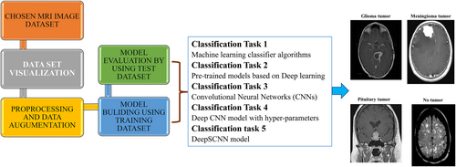
Diagram of the overall workflow employed for classifying brain tumors via MRI scans.
3 METHODS AND MATERIALS
3.1 Dataset
The dataset used in this study was procured from the Kaggle platform (https://www.kaggle.com/datasets/sartajbhuvaji/brain-tumor-classification-mri) and comprised 3264 T1-weighted contrast-enhanced brain MRI images.18 The dataset was divided into two primary sections for training and testing, and the images were grouped into four distinct categories: gliomas (926 images), meningiomas (937 images), pituitary gland tumors (901 images), and healthy brain samples (500 images), as delineated in Table 1. Acquisition modalities included the sagittal, axial, and coronal planes. The visual representation and distribution of these tumor types across different imaging planes in the dataset are illustrated in Figures 2 and 3. Note that the number of images differed for individual patients, reflecting the heterogeneity of the dataset.19
| S. no. | Tumor type | Training sample | Testing sample |
|---|---|---|---|
| 1 | Glioma tumor | 826 | 100 |
| 2 | Meningioma tumor | 822 | 115 |
| 3 | Pituitary tumor | 827 | 74 |
| 4 | No tumor | 395 | 105 |
| Total count | 2870 | 394 |
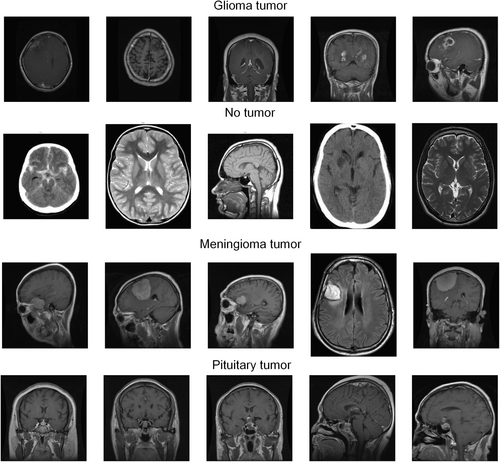
MRI images of brain tumors.
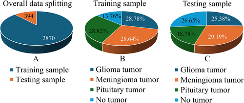
Venn diagram for dataset distribution. (A) Overall data splitting. (B and C) Dataset distribution of each tumor acquired for model building.
3.2 Experimental configuration
Datasets were processed using a personal computer with a 12th Gen Intel Core i7-12700 processor, 16.0 GB RAM, a 64-bit operating system, Conda version 23.5.2, and Python 3.8.17. This setup provided robust computational capabilities and efficient data management.
3.3 Data pre-processing and data augmentation
The first stage of the study involved the processing and enhancement of data, which are crucial steps in preparing the MRI dataset for the training of CNNs.20 Relevant processes included reshaping the pictures into a uniform structure of 15 × 15 matrices with three RGB color channels; pixel values were normalized to (0, 1) to provide numerical stability throughout model training. Contrast stretching was performed to expand the range of gray levels in low-contrast MRI images obtained from various sources and modalities; this was necessary because of artifacts and intensity level discrepancies, requiring machine learning and image processing algorithms for enhancement. Next, data augmentation techniques were introduced to enrich the dataset and prevent overfitting. This included resizing images to standard dimensions of 224 × 224 pixels, rotations of 90°, 180°, and 270° for diverse orientations, and horizontal flipping for dataset variation. Utilizing the flexible ImageDataGenerator function, pixel values were rescaled with options for shearing, zooming, flipping, rotations, shifting, brightness adjustments, and fill mode settings. These extensive data pre-processing and augmentation methods significantly improved the quality and quantity of the dataset, laying a strong foundation for effective medical image analysis and model development.
3.4 Classification tasks based on different models
3.4.1 Task 1: Machine learning classifier models
In the first machine learning classifier task, we employed a diverse set of machine learning classification models, including SVM, random forest classifiers, gradient boosting classifiers, and eXtreme Gradient Boosting (XGBoost) classifiers. Each model was trained on a standardized training set, and predictions were made for the testing set. For training, the dataset was prepared by converting labels and data into NumPy arrays. To enhance the comparability of the models, the data were standardized using the Standard Scaler from Scikit-learn.21
3.4.2 Task 2: Deep learning-based pre-trained classifier models
A suite of deep learning-based pre-trained models, including VGG19, MobileNet, DenseNet169, and InceptionV3, were fine-tuned for the brain tumor image classification task.15 These models were compiled with categorical cross-entropy loss and the Adam optimizer; training involved 50 epochs with early stopping. Evaluation functions were implemented to assess the performance of each model, encompassing classification reports, confusion matrices, and test accuracy. The recorded training histories were used for comparative analysis of the model and to identify the best-performing model based on accuracy.
3.4.3 Task 3: Deep learning-based CNN model
For this task, images were classified using a CNN based on the TensorFlow and Keras open-source software libraries.18, 22 The CNN architecture, essential to the model's performance, was developed layer-by-layer with precise requirements. The network first gathered complex spatial data using a 3 × 3 convolutional layer with 32 filters and rectified linear unit (ReLU) activation. To prevent overfitting, a dropout layer with a rate of 0.2 was carefully included. Next, a 5 × 5 convolutional layer with 64 filters, batch normalization, and a 2 × 2 max-pooling layer were implemented to maintain spatial dimensions by padding. The resilience of the model was further improved using a dropout rate of 0.25. An extra 3 × 3 convolutional layer with 64 filters, batch normalization, and max-pooling was added to the design to improve hierarchical feature extraction. The overfitting resistance was ensured by incorporating a dropout layer with a rate of 0.3. The convolutional layers flattened their output, which was then fed into a dense layer of 512 neurons with ReLU activation to help learn complex relationships in the input. Overfitting issues were further moderated using a 0.4 dropout layer. The final layer had four nodes that corresponded to the four categories in the classification task and used SoftMax activation. After defining the architecture, the model was assembled with the Adam optimizer, employing a categorical cross-entropy loss function tailored for multiclass classification. Training was conducted across 50 epochs with a batch size of 50. Early stopping conditions, triggered by validation loss exceeding a predetermined patience period, halted training to prevent overfitting.
3.4.4 Task 4: Deep learning-based deep CNN (DeepCNN) model with hyperparameter tuning
The Deep learning-based deep CNN (DeepCNN) model was applied for the multiclass classification of brain tumor MRI images, and its hyperparameter was automatically optimized using a grid search algorithm to select the best CNN architecture.13 The architecture comprised six successive convolutional layers, each varying in filter width and kernel diameter. The initial two convolutional layers employed ReLU activation with 64 filters and a (6, 6) kernel. Subsequent layers utilized ReLU activation alongside the (4, 4) and (3, 3) kernels, featuring 128 and 256 filters, respectively. Max-pooling layers with a (2, 2) pool size facilitated spatial downsampling and were applied after every convolutional level. To address overfitting, a dropout layer with a 0.4 rate was followed by a dense layer with 512 units, enabling feature extraction with ReLU activation. The three fully connected layers incorporated kernel regularization with an L2 regularization coefficient of 0.0001, each comprising 512 units with ReLU activation. The output layer consisted of four units with a SoftMax activation function tailored for a specific classification task. The resulting neural network architecture systematically processed and extracted hierarchical features from the input photos, enabling SoftMax-based categorization. An accompanying table details the layer configurations and parameter settings, providing a comprehensive guide for replicating and comprehending these methodologies in picture categorization. To optimize the CNN architecture and training dynamics for image classification, a thorough investigation of hyperparameters was conducted. The strategic exploration ranges for hyperparameters encompass a wide array of architectural arrangements and training approaches. Variations in the number of fully connected and convolutional layers from 1 to 4 offered flexibility in network depth. The range of filters spanned from 16 to 128, providing ample options for feature extraction power, whereas filter sizes from 3 to 7 accommodated diverse receptive fields. Using multiple activation functions, such as exponential linear unit, scaled exponential linear unit (SELU), ReLU, and leaky ReLU, offered a thorough analysis of the nonlinearities. Moreover, using dropout rates of 0.1, 0.2, 0.3, and 0.4 contributed to regularization throughout the training process.
3.4.5 Task 5: Deep learning-based siamese CNN (DeepSCNN)
DeepSCNN has been used to classify dementia stages from MRI images, showing superior performance in diagnosing Alzheimer's disease, even with a small dataset.17 Briefly, the DeepSCNN model contains multiple layers. DeepSCNN begins with convolutional layers, each equipped with ReLU activation for nonlinearity. Batch normalization was employed after Conv1 and Conv3 to stabilize and expedite the training. The max-pooling layers follow Conv2, Conv4, Conv8, and Conv11, strategically reducing the spatial dimensions to effectively capture essential features. Throughout the network, Gaussian noise was applied to enhance robustness against overfitting. The convolutional layers progressively deepen the network's understanding of visual features, culminating in a rich representation of the input image. Max-pooling operations further downsample the feature maps and enhance computational efficiency while preserving crucial information. Layers are flattened by preparing the data for integration, allowing the network to effectively fuse information from different stages. Fully connected layers, FC1 and FC2, with 4096 neurons each, and ReLU activation provide the network with the capacity to learn complex relationships within the feature space. Finally, the SoftMax layer assigns probabilities to each class, producing the final segmentation output. The resulting DeepSCNN model offers an adjustable framework for capturing the distinct traits of various brain tumor images (Figure 4).
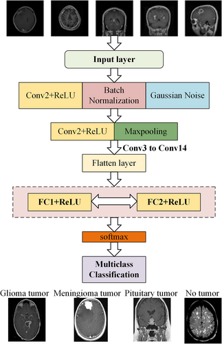
Schematic diagram of the DeepSCNN architecture.
3.5 Performance evaluation
“True Positive” () denoted a sample correctly classified as belonging to the positive class.
“False Positive” () indicated a sample inaccurately classified as belonging to the positive class while actually belonging to the negative class.
“True Negative” () represented a sample correctly identified as belonging to the negative class.
“False Negative” () represented a sample incorrectly categorized as belonging to the negative class while actually belonging to the positive class.
4 RESULTS
4.1 Data pre-processing and data augmentation
The MRI dataset was subjected to thorough pre-processing and augmentation to enhance both the quality and quantity of the data. Gray levels showed an increase through contrast stretching, whereas techniques for data augmentation enhanced uniformity and minimized overfitting. These steps were taken to ensure the dataset's resilience in training CNNs and capturing intricate patterns and features among medical images (Figure 5).
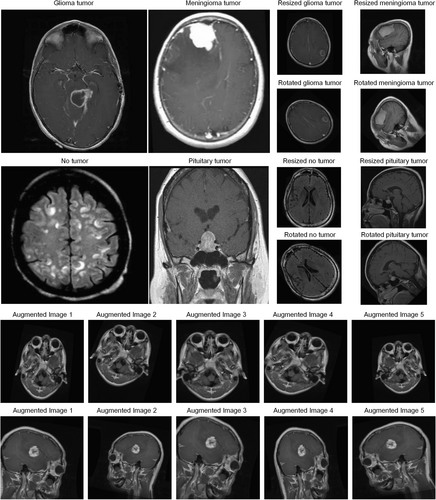
Images generated using data pre-processing and augmentation.
4.2 Classification task 1: Models for machine learning classifiers
Four types of machine learning algorithms were utilized to tackle a specific task in the field of machine learning, each demonstrating distinct levels of performance. As shown in Table 2, the SVM achieved an accuracy rate of 83.62%, demonstrating its ability to effectively handle complex decision boundaries. Random forest, an ensemble model, outperformed this with an accuracy rate of 85.02%, harnessing the predictive capabilities of multiple decision trees. Gradient boost achieved an accuracy rate of 84.32%, relying on continual enhancement of the model accuracy by addressing past shortcomings. The XGBClassifier emerged as the top-performing model, achieving an accuracy rate of 85.89%, highlighting its proficiency in utilizing gradient boosting techniques for enhanced predictive abilities.
| S. no | Machine learning models | |
|---|---|---|
| Model | Accuracy | |
| 1. | Support vector classifier | 0.8362 |
| 2. | Random forest | 0.8502 |
| 3. | Gradient boost | 0.8432 |
| 4. | XGBoost | 0.8589 |
4.3 Classification task 2: Pre-trained classifier models based on deep learning
Using a structured method for image categorization, numerous pre-trained models were fine-tuned using Keras ImageDataGenerator for data preparation. In addition, augmentation methods were implemented in the training set. Multiple models, such as VGG19, MobileNet, DenseNet169, and InceptionV3, were chosen and configured with categorical cross-entropy loss and the Adam optimizer. The training procedure lasted for 50 epochs with integrated early stopping. The accuracy outcomes are presented in Table 3. These findings form a thorough basis for selecting the most efficient pre-trained model and assessing loss and accuracy metrics within the specific context of image classification.
| S. no | Pre trained deep learning models | |
|---|---|---|
| Model | Accuracy | |
| 1 | VGG19 | 0.7208 |
| 2 | MobileNet | 0.7665 |
| 3 | DenseNet169 | 0.7487 |
| 4 | InceptionV3 | 0.7030 |
4.4 Classification task 3: CNN model based on deep learning
In the third classification task, the CNN model reported precision scores of 0.89, 0.79, 0.83, and 0.99 for the no-tumor, glioma tumor, meningioma tumor, and pituitary tumor categories, and the corresponding F1-scores were 0.82, 0.86, 0.83, and 0.90, respectively. The proposed model achieved an overall accuracy of 0.87. Notably, the model exhibited high recall for glioma and pituitary tumor classes, underscoring its effectiveness in identifying these specific tumors (Table 4 and Figure 6).
| Hyper parameter | Range of parameters | Optimum value |
|---|---|---|
| Num_conv_layers | (1, 2, 3, 4, 5, 6) | 6 |
| Num_fc_layers | (1, 2, 3, 4) | 3 |
| Num_filters | (16, 24, 32, 48, 64, 96, 128,256) | [64, 64, 128, 128, 256, 256] |
| Filter_size | (3, 4, 5, 6, 7) | [6, 6, 4, 4, 3, 3] |
| Activation_func | (ELU, SELU, ReLU, leaky ReLU) | “ReLU” |
| Dropout_rate | (0.1, 0.2, 0.3, 0.4) | 0.3 |
| Num_maxpool_layers | (1, 2, 3, 4, 5, 6) | 6 |
| Mini_batch_size | (4, 8, 16, 32, 64) | 32 |
| Learning_rates | (0.0001, 0.0005, 0.001, 0.005) | 0.005 |
| L2_regs | (0.0001, 0.0005, 0.001, 0.005) | 0.001 |
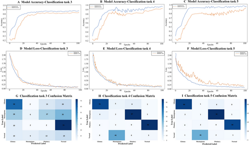
Accuracy and loss curves, as well as the confusion matrix, for classification tasks 3, 4, and 5.
4.5 Classification task 4: Deep CNN model with hyperparameter tuning
Through a rigorous examination of the effects of various hyperparameters on the performance of our CNN model during the intricate optimization process, we identified the most effective configuration which is presented in Table 5.
| Classification task | Classes | Precision | Recall | F1-score | Test accuracy |
|---|---|---|---|---|---|
| Classification Task 3 - CNN model based on deep learning | No tumor | 0.89 | 0.77 | 0.82 | 0.87 |
| Glioma tumor | 0.79 | 0.93 | 0.86 | ||
| Meningioma tumor | 0.83 | 0.84 | 0.83 | ||
| Pituitary tumor | 0.99 | 0.85 | 0.9 | ||
| Classification Task 4 - deep CNN model with hyper parameter tuning | No tumor | 0.89 | 0.95 | 0.94 | 0.94 |
| Glioma tumor | 0.98 | 0.89 | 0.87 | ||
| Meningioma tumor | 0.91 | 0.98 | 0.94 | ||
| Pituitary tumor | 0.99 | 0.94 | 0.97 | ||
| Classification Task 5 - deep learning based deep siamese convolutional neural network (DeepSCNN) | No tumor | 0.96 | 0.98 | 0.97 | 0.96 |
| Glioma tumor | 0.97 | 0.92 | 0.95 | ||
| Meningioma tumor | 0.94 | 0.96 | 0.95 | ||
| Pituitary tumor | 0.99 | 0.98 | 0.96 |
Following extensive trial and error, we determined that the optimal configuration consists of three convolutional layers and three fully connected layers. This configuration enables the model to efficiently capture hierarchical features without becoming overly complex. Achieving the best configuration of (64, 64, 128, 128, 256, and 256) involves gradually increasing the number of filters to refine the evolution of the convolutional layers. This incremental adjustment plays a vital role in enhancing the capability of the model to detect intricate hierarchical structures within the data. The choice of filter size was also critical, with optimal values of,3, 6 emphasizing the importance of utilizing medium-sized filters. The most effective activation function was ReLU, indicating the usefulness of introducing nonlinearity and aiding the model in recognizing complex correlations within the data. In terms of regularization, we determined that a dropout rate of 0.3 is optimal. This rate of regularization significantly improved the generalizability of the model by preventing overfitting. Establishing three max-pooling layers as the best configuration underscores the significance of hierarchical feature reduction in enhancing the abstraction capabilities of the model. Furthermore, an ideal mini-batch size of 32 was determined for efficient resource utilization and convergence balance. The learning dynamics of the model are sensitive to the chosen parameter update rate, with a learning rate of 0.005 proving to be the most effective for achieving optimal convergence. The inclusion of L2 regularization at a rate of 0.001 is also crucial for reducing the risk of overfitting and enhancing the model's generalization capabilities, as illustrated in Table 6.
| S. no | Model classifiers | Accuracy |
|---|---|---|
| 1. | XGB classifier | 0.85 |
| 2. | MobileNet | 0.76 |
| 3. | CNN model | 0.87 |
| 4. | Deep CNN model | 0.94 |
| 5. | DeepSCNN | 0.96 |
- Note: The highlights demonstrated our model's superior performance using state-of-the-art techniques. Common in research articles to high-light major results as bold.
In classification task 4, precision values ranged from 0.87 to 0.99 for the no-tumor, glioma tumor, meningioma tumor, and pituitary tumor classes, and the F1-scores ranged from 0.87 to 0.97. The recall values for tumor classification ranged from 0.89 to 0.98, with meningioma exhibiting the highest recall of 0.98, followed by no tumor with 0.95 and pituitary tumor with 0.94. These metrics, along with an overall accuracy of 0.94, underscored the effectiveness of the model in accurately classifying tumor types in task 4 (Table 6 and Figure 6).
4.6 Classification task 5: DeepSCNN model
In classification task 5, the proposed DeepSCNN model demonstrated outstanding performance in classifying brain tumor images; high metrics were achieved across multiple evaluation criteria. The model was trained and tested on a comprehensive dataset including the four distinct classes: no tumor, glioma tumor, meningioma tumor, and pituitary tumor. The overall accuracy of the DeepSCNN model was 96%. This indicates that the model correctly classified the vast majority of the images in the dataset. The high accuracy is a testament to the architecture's robustness and effectiveness in capturing and understanding the intricate features of brain tumor images. In terms of precision, the model excelled across all tumor types. The precision scores were 0.96 for no tumor, 0.97 for glioma tumors, 0.94 for meningioma tumors, and 0.99 for pituitary tumors. These high values suggest a low false-positive rate. Thus, the model performed well with minimal misclassification in identifying the presence or absence of tumors. Sensitivity or recall, which measures a model's ability to correctly identify true positives, also reflects its effectiveness. Notable improvements were observed in the recall scores, particularly for the no-tumor and meningioma tumor classes. This indicates that the DeepSCNN model would be proficient in detecting actual tumor cases, with a low likelihood of missing existing tumors. Moreover, the F1-score, which balances precision and recall, showed significant improvements compared with other models for the no-tumor and meningioma tumor classes, highlighting the model's overall balanced performance in identifying these tumor types (Table 6 and Figure 6).
Of the four machine learning algorithms, the XGBClassifier achieved an accuracy of 0.85, whereas the pre-trained deep-learning MobileNet reached 0.76. A CNN model recorded an accuracy of 0.87, and a deep CNN model with hyperparameter tuning achieved 0.94. Notably, our DeepSCNN model outperformed the others with a high accuracy of 0.96. Performance evaluation metrics, such as accuracy and precision, were computed using standard measures for model evaluation.
5 DISCUSSION
Accurate brain tumor classification is critical for the diagnosis and treatment of brain cancers but remains challenging owing to the complexity of tumor types. This study evaluated the performance of five state-of-the-art tumor classification models, including our newly proposed model, DeepSCNN. The results are shown in Table 4, indicating that the DeepSCNN architecture is more robust and suitable for image classification tasks.
Previous research has evaluated these models against random forest and SVM algorithms, achieving an area under the curve of approximately 80%.7, 11, 19 Deep learning algorithms, such as simple CNNs24 and the proposed DeepCNN, have been employed for brain tumor classification and exhibited AUCs of 85% and 94%, respectively.14, 18, 20, 25 Various types of transfer learning have been used to classify brain cancers with high accuracy, as reported in multiple studies.10, 23, 26, 27 Our research focuses on the multiclass classification of brain tumors using DeepSCNN; a similar architecture was shown to be effective in classifying stages of Alzheimer's disease.17
Our analysis confirmed that DeepSCNN outperformed the other classifier categories (Table 4) and existing systems (Table 7), demonstrating higher precision and accuracy30-34 because of its architectural components, including the use of convolutional layers for hierarchical feature learning, batch normalization for enhanced stability and accelerated convergence, and Gaussian noise for regularization against overfitting. Additionally, the model employs max-pooling layers to effectively reduce spatial dimensions while retaining key information, and fully connected layers with large neuron counts help capture complex relationships within the data. As a result, the DeepSCNN architecture is not only more effective in accurately classifying brain tumors but also promising for classifying other brain disorders.15
| S. no | Model | F1 score | Accuracy |
|---|---|---|---|
| 1. | KNN27 | - | 91.10% |
| 2. | DeepCNN13 | - | 92.66% |
| 3. | MCNN28 | 0.91 | - |
| 4. | CNN29 | 0.93 | 94.39% |
| 5. | Our model DeepSCNN | 0.96 | 96.00% |
- Note: The highlights demonstrated our model's superior performance using state-of-the-art techniques. Common in research articles to high-light major results as bold.
- Abbreviations: KNN, K-Nearest Neighbors; MCNN, Multi-Scale CNN.
Despite these encouraging results, our study has some limitations. The proposed framework must be validated in broader clinical trials to ensure its robustness and generalizability across diverse patient populations.31-35 Additionally, the decision-making process in deep learning models remains complex and lacks transparency.36 Future research should integrate explainable AI methods to improve interpretability, providing clearer insights into model decisions, especially for multimodal and multi-center data.37, 38 Enhancing interpretability and validating the framework remain crucial areas for future work.
6 CONCLUSION
In the use of MRI for brain tumor classification, accuracy is crucial for early detection and precise categorization. Enhanced accuracy contributes to better treatment planning and patient outcomes. To support this, we investigated five different models for brain tumor classification and compared their performance for neuro-oncology diagnostics. Our results indicate that DeepSCNN is the highest-performing model for the classification of brain tumors. Ultimately, when successfully developed and implemented, DeepSCNN may significantly improve patient outcomes in neuro-oncology. Its performance and design should be further examined to support its application as a powerful tool in medical diagnostics.
AUTHOR CONTRIBUTIONS
Gowtham Murugesan: Conceptualization; methodology; software; formal analysis; investigation; data curation; visualization; writing—original draft; writing—review and editing. Pavithra Nagendran: Methodology; formal analysis; visualization; writing—review and editing. Jeyakumar Natarajan: Conceptualization; investigation; supervision; and writing—review and editing.
ACKNOWLEDGMENTS
The authors received no specific funding for this work.
CONFLICT OF INTEREST STATEMENT
The authors declare no conflicts of interest.
ETHICS STATEMENT
The dataset was procured from the Kaggle platform (https://www.kaggle.com/datasets/sartajbhuvaji/brain-tumor-classification-mri), so ethics approval was not needed in this study.
Open Research
DATA AVAILABILITY STATEMENT
All data generated or analyzed during this study are included in this published article. The link of the public MRI dataset that is used in this study is: https://www.kaggle.com/datasets/sartajbhuvaji/brain-tumor-classification-mri.


