Carbon balances of bioenergy systems using biomass from forests managed with long rotations: bridging the gap between stand and landscape assessments
Abstract
Studies report different findings concerning the climate benefits of bioenergy, in part due to varying scope and use of different approaches to define spatial and temporal system boundaries. We quantify carbon balances for bioenergy systems that use biomass from forests managed with long rotations, employing different approaches and boundary conditions. Two approaches to represent landscapes and quantify their carbon balances – expanding vs. constant spatial boundaries – are compared. We show that for a conceptual forest landscape, constructed by combining a series of time-shifted forest stands, the two approaches sometimes yield different results. We argue that the approach that uses constant spatial boundaries is preferable because it captures all carbon flows in the landscape throughout the accounting period. The approach that uses expanding system boundaries fails to accurately describe the carbon fluxes in the landscape due to incomplete coverage of carbon flows and influence of the stand-level dynamics, which in turn arise from the way temporal system boundaries are defined on the stand level. Modelling of profit-driven forest management using location-specific forest data shows that the implications for carbon balance of management changes across the landscape (which are partly neglected when expanding system boundaries are used) depend on many factors such as forest structure and forest owners’ expectations of market development for bioenergy and other wood products. Assessments should not consider forest-based bioenergy in isolation but should ideally consider all forest products and how forest management planning as a whole is affected by bioenergy incentives – and how this in turn affects carbon balances in forest landscapes and forest product pools. Due to uncertainties, we modelled several alternative scenarios for forest products markets. We recommend that future work consider alternative scenarios for other critical factors, such as policy options and energy technology pathways.
Introduction
Assessing greenhouse gas (GHG) balances and the climate effects of bioenergy is essential to inform policy development and implementation. Studies that assess GHG balances for bioenergy systems sometimes assume that bioenergy systems are neutral in regard to the biosphere–atmosphere CO2 flows, since the bioenergy system is integrated in the carbon cycle and carbon sequestration and emissions balance over a full growth-to-harvest cycle. It is, however, well established that bioenergy systems can influence the cycling of carbon between the biosphere and the atmosphere (Smith et al., 2014). The timing and magnitude of carbon emissions and sequestration associated with forest-based bioenergy have received much attention in recent years. Studies report different findings, in part due to varying scope and use of different approaches to quantify GHG and carbon balances.
Forest carbon balances are quantified using a range of methodologies, and the appropriate spatial and temporal scales for meaningful analysis are key. In countries where even-aged forestry dominates and thus, most of the trees are harvested in a ‘final felling’ at the end of the rotation period, one spatial scale considered for carbon balance calculations is the forest stand, that is, the typical scale for final-felling operations. Studies using stand-level calculations typically consider carbon balances over one or several rotation periods; the growing stand sequesters carbon until it is released into the atmosphere by either biomass decay or combustion, so there will always be a difference in timing of carbon emissions and sequestration. Stand-level analyses often focus on assessing the carbon balance associated with specific operations such as forest thinning or residue collection for bioenergy at final felling (see e.g. Schlamadinger et al., 1995; Schlamadinger & Marland, 1996; Cherubini et al., 2011; Helin et al., 2013; Holtsmark, 2013).
Where management activities are coordinated across the whole landscape to obtain a continuous flow of wood for the forest industry, calculating carbon balance at the landscape scale can be more appropriate (Eliasson et al., 2013; Cintas et al., 2016). The large shifts observed at the stand level, from net carbon sequestration to net carbon emissions at harvest, are not observed at the landscape level. Carbon losses in some stands are balanced by carbon gains in other stands, so that across the whole forest landscape the carbon stock follows a trend line that can be increasing or decreasing, or roughly stable over time. The intuitive conclusion from this, that stand-level and landscape-level assessments of the carbon balance of forest bioenergy will yield different results, has been confirmed by various studies (see, e.g., Galik & Abt, 2012; Berndes et al., 2013; Cintas et al., 2016), but has also been challenged by Cherubini et al. (2013) who found that assessments at the stand and landscape scales yielded the same results.
The relevant temporal system boundaries of an assessment depend on its purpose. Both the time period for accounting and the time at which accounting is commenced, relative to the first harvest for bioenergy, influence the outcome (Berndes et al., 2013). Stand-level assessments sometimes start carbon accounting at the time of the first biomass extraction for bioenergy, commencing with a pulse emission followed by a phase of sequestration; net GHG savings are therefore often only achieved after a period of time. These studies have been criticized as ‘…based on the unrealistic assumption that trees are first burned and then grown…’ (WBA, 2012). However, if the purpose of the study is to investigate the effects of introducing biomass extraction for energy as a new component in the management of an existing forest, then the motivation for using this approach can be valid. On the other hand, if the purpose is to investigate the climate effects of incentivizing bioenergy, the definition of time period for accounting is less clear since land owners and other actors in the forest sector can respond to bioenergy incentives in many different ways and forest management might be adapted to anticipated bioenergy demand in advance of the first biomass extraction and use for bioenergy. Due to this, it might be considered appropriate to start the accounting clock earlier, for example, at the time when forest management is adapted to anticipated bioenergy demand (Cowie et al., 2013).
Studies that intend to support policy development and strategic considerations need to address the question of how changes in forest carbon stocks at the landscape scale resulting from bioenergy incentives affect GHG impacts of bioenergy implementation over time (Cowie et al., 2013; Miner et al., 2014). Assessment at the landscape scale integrates the effects of all changes in the forest management and harvesting regime that take place in response to – experienced or anticipated – bioenergy demand. Taken together, these changes may have a positive, negative or neutral influence on the development of forest carbon balances. For example, Galik & Abt (2012) compared six different assessment scales and four different metric calculation techniques against the backdrop of a common biomass demand scenario. They found that those assessments that did not include market effects attributable to increased biomass demand, including changes in forest area, forest management intensity and traditional industry production, generally produced higher net GHG emissions than those that do.
A forest landscape can be simply represented by a series of time-shifted stands. The ideal forest landscape has the same number of stands as the number of years in the rotation period; at any point in time, the forest landscape has a uniform age distribution, consisting of even-aged and even-sized stands (cf. Cherubini et al., 2013; Eliasson et al., 2013; Jonker et al. 2014; Helin et al. 2016). In this paper, such hypothetical forest landscapes are designated as ‘conceptual landscapes’. One reason studies quantify carbon balances in conceptual landscapes rather than using ‘real’ forest landscapes is that it is relatively easy and can be used to illustrate how specific factors affect outcomes, for example, the influence of a change in average rotation period on forest carbon stocks, or of establishment of new practices such as stump harvesting at final felling.
Alternatively, location-specific data and models can be used to assess carbon balances in specific ‘real landscapes’, which generally have unequal distributions of age classes and stands of different sizes. They also usually contain non-harvested areas, such as riparian buffers and habitat conservation areas, which should be excluded from the analysis so that they do not skew the assessment of forest management impacts on forest carbon balances. Ideally, assessments should consider that forest management planning supports the production of a variety of forest products with different GHG balances depending on factors such as fossil carbon displacement efficiency (the carbon emissions avoided as a consequence of using the forest products), forest age class distribution, varying site conditions, interrelation among forest products (Melin et al., 2010; Hudiburg et al., 2011; Lundmark et al., 2014; Kilpeläinen et al., 2016) and market effects (cf. Abt et al., 2012; Nepal et al., 2012; Sedjo & Tian, 2012). Further, biomass demand for energy affects landowner decisions and the interrelations among forest product outputs. Landowners may intensify forest management or expand forest areas based on an expectation that future biomass demand will be higher, or they may abstain from converting forest to other land use, for example, pasture production (cf. Miner et al. 2014).
This paper considers different approaches to calculating carbon balances for bioenergy systems that use biomass from forests that are managed with long rotations to produce multiple forest products. It builds on the analytical framework used in Cintas et al. (2016) and complementary modelling for scaling up the stand level to conceptual landscape level. We show how different approaches to quantify carbon balances in the same conceptual forest landscapes can yield different conclusions depending on how system boundaries are set. Further, we model real landscapes to show that carbon balances for different bioenergy systems can vary significantly depending on market development for other forest products. Since the focus is on comparing and discussing methodological choices in carbon balance calculations, non-CO2 climate forcers and supply-chain emissions are not considered. Risks and consequences of storms, wildfires, forest pests and diseases are also not considered in this study, although we acknowledge that such events can have a strong influence on net carbon balances (cf. Buchholz et al., 2015).
Materials and methods
Model representation of forest management and the production and use of forest products
The Q model (Ågren et al., 2008; Eliasson et al., 2013) is used to quantify annual carbon balances for forest stands and conceptual forest landscapes subject to varying harvest intensities (see scenarios in Table 1). The forest stand is modelled as an even-aged stand established through planting. The conceptual forest landscape is generated by combining time-shifted single stands to obtain an ideal forest landscape consisting of stands of equal area with all ages represented (i.e. for 100-year rotation length, the forest consists of 100 stands of equal area, planted consecutively over 100 years). The landscape is assumed to have a homogeneous site quality, that is, stands that are subject to the same management have identical growth development and carbon balance. Each year the oldest stand is harvested and becomes a newly planted re-growing stand the subsequent year.
| Scenario | Harvest |
|---|---|
| REF | Stemwood from all thinning operations and from final felling |
| REF_NT | Stemwood from final felling |
| BIOC | REF + 80% of slash (tops and branches) from all thinning operations and from final felling |
| BIOC_NT | REF + 80% of slash from final felling |
The Heureka PlanWise software (Wikström et al., 2011) is used to quantify the carbon balance in real Swedish forest landscapes that are subject to forest management planning to meet expected demands for forest products (see Scenarios in Table 2). PlanWise is an optimization application within the Heureka decision support system that supports forest management planning relating to timber production, profit, environmental conservation, recreation and carbon sequestration (Wikström et al., 2011). Forecasts are based on growth models (Fahlvik et al., 2014) as well as mortality and in-growth models to consider growth of naturally regenerated seedlings in-between the already established trees.
| Scenario | Price of wood products and management | Harvest for bioenergy (all scenarios include harvest of sawtimber and pulpwood) |
|---|---|---|
| Reference | ||
| BAU | Constant price trend for sawnwood and pulpwood. Bioenergy is not factored into the management plan | Slash is extracted when the volume of spruce is at least 60% of the total volume in the stand subject to final fellinga. Slash is extracted in about 40% of the final felling |
| BAUdpulp | Same as BAU but with linear decrease in pulpwood price to become 75% less than BAU after 100 years | |
| Bioenergy | ||
| BIO | Same as BAU but with bioenergy factored into the forest management (constant price trend also for bioenergy) | Slash is extracted when the volume of spruce is at least 20% of the total volume in the stand subject to thinning or final felling. Slash is extracted in about 45% of the thinnings and about 60% of the final fellings |
| BIO+ | Same as BIO but with linear increase in bioenergy price to reach 100% higher than BAU after 100 years. Fertilization and genetically improved seedlings enhance growth | |
| BIOdpulp | Same as BIO but with linear decrease in pulpwood price to become 75% less than BAU after 100 years, that is, declining demand for pulpwood | |
| BIOdpulp75 | Same as BIOdpulp | Same as BIOdpulp but reallocating a linearly increasing share (from 0% to 75%) of the pulpwood to bioenergy use |
- a Spruce produces more slash than pine, and therefore, extraction from spruce dominated forests is economically more suitable.
The CAfBio model is used to quantify carbon flows and storage in forest products until the point in time when the carbon is released to the atmosphere. The harvested biomass is allocated to the production of forest products (different forest products are assumed in different scenarios, see below). The residence time for carbon in the forest products pool is modelled using the gamma decay function in Earles et al. (2012). The carbon in discarded forest products is either emitted to the atmosphere via incineration, transferred to new products via recycling or transferred to landfill, assuming a degradable organic carbon fraction of 0.5, methane correction factor of 0.95, methane generation rate of 0.04 for paper, and 0.02 for wood waste, following Supporting information in Earles et al. (2012). The modelling output is expressed in terms of the carbon balances associated with the forest products, including avoided carbon emissions due to displacement of fossil fuels and other products, for example, concrete. For more details, see Cintas et al. (2016).
Approaches to carbon accounting
The stand-level accounting is set to start at the time of final felling and biomass extraction, in order to produce a carbon balance profile characterized by initial carbon emissions followed by carbon sequestration. Two approaches are used for the conceptual landscape:
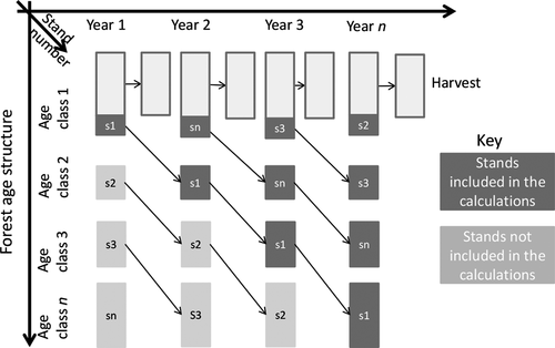
The expanding spatial boundary (ESB) approach [equivalent to the method of Cherubini et al. (2013)] combines the outcome of the stand-level carbon accounting for an increasing number of separate forest stands. To generate an ideal forest landscape, ESB expands the spatial boundary by including one new stand ready to be harvested each year (see Cherubini et al. (2013) and Fig. 1). The total number of individual stands brought into the system equals the number of years in the forest rotation, an approach equivalent to the ‘increasing stand-level’ approach of Jonker et al. (2014).
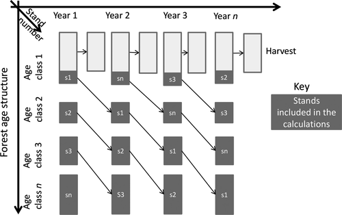
The constant spatial boundary (CSB) approach accounts for carbon emissions and sequestration across the whole landscape throughout the accounting period [see Fig. 2 and Eliasson et al. (2012)]. The spatial system boundary does not change over time, and emissions/sequestration in different stands balance out. For the ideal forest landscape, with a sustained-yield harvest (i.e. the annual harvest is equal to the annual growth), the CSB approach will show a steady-state situation with stable landscape carbon stock. In a forest in a transition state, forest management is changed from historical management to a new management regime (e.g. if forest owners start collecting slash previously left on site). CSB accounting reflects how the management changes affect the carbon stock in the whole landscape over time.
Scenarios and parameterization of forests and forest management
Single stands and conceptual landscapes
The forest scenarios REF and BIOC presented in Table 1 are based on Eliasson et al. (2013). The parameterization is representative of Norway spruce stands in southern Sweden (with a site index of G26 near Växjö; 56.87°N, 14.81°E) with a rotation period of 100 years. REF represents a common Swedish management plan, with three thinnings (at 33, 48 and 65 years) and final felling at 100 years. BIOC represents a practice that extracts slash (i.e. tree tops and branches) at each cutting, for bioenergy. Two other scenarios, REF_NT and BIOC_NT, are adapted from REF and BIOC to represent similar situations but without thinning operations (‘NT’ for ‘no thinning’). Current real forestry practices include thinning, but the ‘NT'_scenarios allow for comparison with studies that only consider final-felling operations. Historic forest management is assumed to be REF, that is, without slash extraction for bioenergy.
All harvested biomass is assumed to be used for energy, to facilitate analyses of the differences between ESB and CSB (this assumption does not reflect the reality in Sweden today). To further facilitate comparisons, bioenergy is assumed to displace natural gas (NG) and coal, as these are commonly used as reference fuels in other studies. Displacement factors are set to 1.27 Mg fossil C per Mg of C in biomass used to displace coal and 0.55 Mg fossil C per Mg of C in biomass used to displace NG (Cintas et al., 2016). The former can be said to represent a situation where a coal-based heat boiler and a coal-based power plant are shut down and replaced with new biomass-based CHP, and the latter represents a situation where new biomass-based CHP is built instead of new gas-based CHP, either to replace old generation or to meet increasing energy demand.
Real forest landscape
Several scenarios (see Table 2) were developed to support the assessment and analysis of forest management in a 9171-ha landscape surrounding Skellefteå (64.5°N) in northern Sweden. The initial average growing stock is 121 m3 ha−1 of 73% Scots pine, 22% spruce and 5% broadleaves (Holmström et al., 2012), with a 3.7 m3 ha−1 yr−1 average production potential and 100-year planning horizon.
The business-as-usual scenario (BAU) simulates forest managed for sawnwood and pulpwood production; forest-based fuels are considered a by-product stream that might be extracted if economic conditions allow, but not considered a relevant factor in management planning. BAU is an update of scenarios presented in Holmström et al. (2012).
Five associated scenarios simulate changes in demand for different wood products: (i) BIO represents an increase in demand for bioenergy, with forest owners adapting their forest management to factor in three products considered equally important: sawnwood, pulpwood and forest-based fuels. (ii) BIO+ is BIO with a stronger market for biofuels. (iii) BAUdpulp is BAU but with pulpwood demand decreasing, represented by the pulpwood price declining over time. (iv) BIOdpulp is BIO but with the same declining pulpwood price as in BAUdpulp. (v) BIOdpulp75 is BIOdpulp, but a percentage of the pulpwood is used as biofuel feedstock (the percentage increases linearly from 0% to 75% in 100 years), representing the pulpwood output not decreasing as much as the price.
The outcome of each scenario corresponds to the best-adapted management in the Skellefteå forest landscape, that is, the most profitable forestry regime providing a continuous flow of sawtimber, pulpwood and biomass for energy over time. An even-flow requirement is included for each forest management plan, which does not force a constant flow of products but ensures inertia against major changes over a 5-year period (i.e. the length of the time steps in the model runs) to avoid unrealistic sudden shifts in forest management. All scenarios simulate forest management activities that potentially involve changes in rotation period, thinning frequency and harvesting intensity at thinnings and final fellings. BIO+ also includes fertilization and the use of genetically improved seedlings. The extraction of slash is simulated in final felling and thinning at the stand-level when some basic criteria are met. These criteria include a minimum percentage of spruce in the stand (see table below), as well as site and soil moisture conditions (no slash extraction is simulated on poor sites with a site index lower than 20 m – expected mean height for dominant trees at the age of 100 years – or when soil moisture is classified as ‘wet’). For all the scenarios, the slash extraction rate is 80% of the available above-ground biomass after stem harvest, assuming that no logging residues are needed to reinforce strip roads [i.e. in moist areas, see upper limit in Nurmi (2007)]. The model also includes the effect of repeated extraction of slash on forest growth [<5% reduction per rotation period, see Helmisaari et al. (2011)]. The forest management practices are economically evaluated to achieve optimal bucking in relation to (i) a real price list for timber, pulpwood and bioenergy defined and used by Mellanskog (a forest owners association in central Sweden) during the first quarter of 2013; and (ii) cost functions for the simulated forest management activities (Brunberg, 2004, 2007; Ackerman et al., 2014). Net present values as a basis for forest management optimization in the given market situation are calculated according to Faustmann (1995), with a discount rate of 2%, representative of Swedish forestry.
The bioenergy scenarios are compared with reference scenarios, BAU and BAUdpulp. The difference in sawtimber production is reflected in the production volume for concrete. The use of wood for structural material is already high in Sweden, but it was nevertheless assumed that the produced sawnwood substitutes concrete because there is significant scope for increased use of sawnwood in multi-storey buildings (Gustavsson et al. 2006). In the bioenergy scenarios, pulpwood production above the level in BAU is used for energy purposes; that is, the same demand for paper products is met in all scenarios. Bioenergy is assumed to displace NG and coal as described above, and sawnwood use is associated with fossil carbon displacement factors at 2.74 and 2.31 Mg fossil C per Mg C in sawnwood, which corresponds to displacement of concrete where either coal or NG was used in the manufacturing process of the displaced concrete, see Cintas et al. (2016).
Forest management choices are based on price trends known beforehand and assume that all the forest owners aim to maximize their profit. The Skellefteå forest landscape was selected because it is privately owned; as pointed out by Miner et al. (2014), private landowners are more sensitive to price signals.
Results
Carbon dynamics in single stands and conceptual landscapes
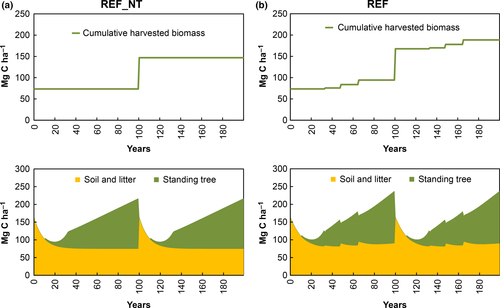
Figure 3 shows the carbon storage in soil and litter and standing trees (designated as ‘forest pools’) at the stand level and carbon in cumulative biomass harvests in REF and REF_NT, for two rotation periods (200 years). In this section, we show how ESB and CSB capture the carbon dynamics at the level of conceptual forest landscapes built by combining forest stands with the carbon dynamics shown in Fig. 3.
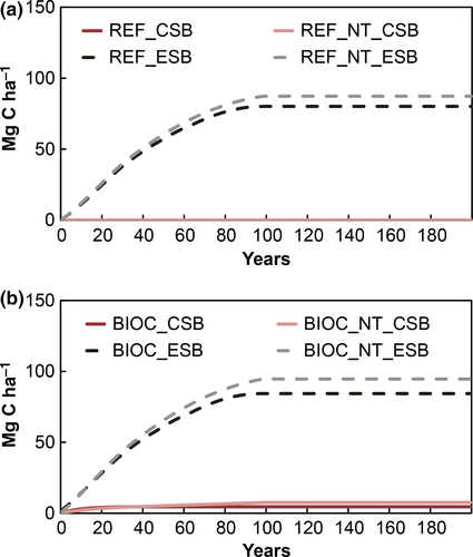
Figures 4 and 5 show the outcome of carbon accounting at the landscape level. For cumulative carbon in harvests, ESB and CSB yield the same results for REF_NT and BIOC_NT (Figs 4a and 5a), while for REF and BIOC a slightly lower result is obtained with ESB (Figs 4b and 5b). The discrepancy is due to ESB ignoring harvests from thinning in those stands that have not yet been subject to final felling (the stands under the diagonal in Fig. 1).
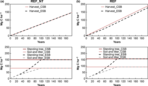
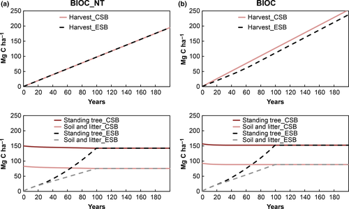
Figures 4 and 5 further illustrate that ESB and CSB yield different results for carbon stored in forest pools. CSB shows constant carbon storage (Fig. 4, managed forest in steady state; managed in the same way as historically) or slightly declining carbon storage (Fig. 5, forest in transition from historic management to a new management regime that includes slash extraction), while ESB shows increasing carbon storage, from zero up to the same level as for CSB after a time period corresponding to one rotation period. ESB includes an increasing number of stands, and hence increasing amounts of carbon stored in the forest pools, during the first rotation period. After one rotation period, the two accounting approaches match each other, for carbon in forest pools, since both then consider all the stands in the forest landscape.
Figure 6a shows the cumulative net carbon flux from the forest landscapes (i.e. the cumulative emissions minus sequestration for each year) in REF and REF_NT. CSB shows the expected outcome when identical forest stands are combined to form a uniformly structured forest that is managed in the same way as it has been historically: emissions and sequestration balance out, and the carbon balance is zero. In contrast, ESB shows an increasing cumulative net carbon flux during the first 100 years (one full rotation period) as stands are gradually included within the system boundary. This is due to that sources of emissions and sequestration in the landscape are gradually included in the accounting. Each year a new stand ready to be felled is added to the landscape; it contributes an initial carbon emission pulse (as the harvested biomass is combusted) followed by carbon sequestration associated with stand re-growth. Emissions (biomass combustion and decay) initially dominate, but as more stands are added to the forest landscape sequestration in re-growing stands increasingly balances the emissions (Fig. 7). Thus, the ESB outcome is initially strongly influenced by the carbon dynamics at the stand level, and there will always initially be a positive carbon balance when stands are assumed to be harvested, and the biomass burned, in the year they are brought into the accounting.
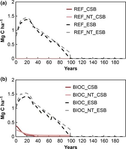
For BIOC and BIOC_NT (Fig. 6b), which represent a transition to a new forest management regime where slash extraction adds to the total biomass harvest, CSB initially shows an increase in the cumulative net carbon flux as slash previously left in the forest is instead harvested and used for energy. The net carbon flux approaches zero as the forest landscape approaches a new steady state. In BIOC_NT, this state is reached after the first rotation period when all stands are subject to the new management regime (Fig. 7b). In BIOC, the net carbon flux becomes zero after a few decades, when the new management regime is implemented in the whole landscape, that is, when all stands have been subjected to either final felling or thinning, and carbon emissions and sequestration are the same. Note that when slash is harvested at thinnings, the new harvest intensity is implemented in the stand. With ESB, the results for the bioenergy scenarios are similar to those for REF and REF_NT, since the influence of the stand-level dynamics masks the effect of the management transition.
Net GHG balance of increased harvest for bioenergy in the conceptual landscape
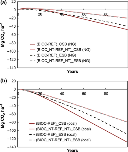
The cumulative net GHG balance of increasing the biomass harvest to displace fossil fuels can be calculated by adding the fossil GHG emissions reduction to the calculated difference in cumulative net carbon flux between a bioenergy scenario and reference scenario. As seen in Fig. 8, the ESB and CSB approaches yield the same results if biomass is only harvested at the final felling (BIOC_NT-REF_NT), but not when biomass from thinning operations is included (BIOC-REF). This is due to that ESB ignores stands that have not yet been subject to final felling, that is, both growth and harvest associated with thinning in those stands are ignored.
Carbon dynamics in real landscape scenarios
Almost all bioenergy scenarios have less carbon in the forest pools than the corresponding reference scenarios throughout the time period (Fig. 9). The biomass harvest is consistently larger in the bioenergy scenarios, and the cumulative difference in biomass harvest is larger (and growing) than the forest pool difference. As expected, bioenergy adaptation of forest management consistently leads to a much larger percentage change in residue harvest than in sawtimber and pulpwood production (Fig. 10).
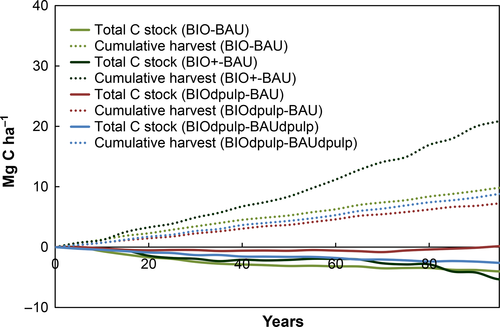
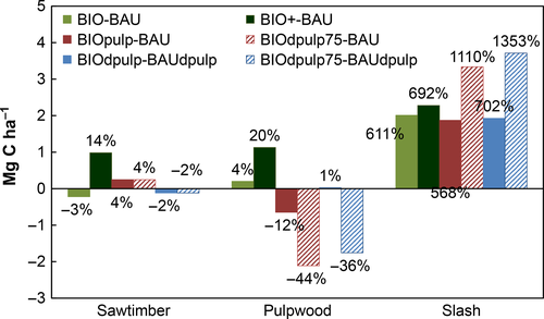
In a scenario with a constant price trend for sawnwood and pulpwood (BAU), adding consideration of bioenergy (BIO) in the forest management planning leads to slightly shorter rotation periods, about 4% more pulpwood production and about 3% less sawtimber production. The amount of slash harvested for bioenergy is about 600% higher (Fig. 10), while carbon storage in the forest pool is lower in BIO than in BAU (Fig. 9). The reduction in forest carbon stock outweighs the fossil GHG savings during the first 45 years when bioenergy displaces NG, while immediate net GHG savings are achieved when bioenergy displaces coal (Fig. 11).
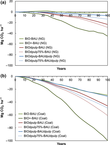
When bioenergy demand is larger and bioenergy prices are higher (BIO+), more intensive forestry including more fertilization and the use of genetically improved seedlings is implemented. Average rotation periods become shorter (91 years compared to 105 years) and biomass output increases (sawtimber +14%, pulpwood +20% and forest fuel +700%) (Fig. 10); more carbon is stored in the forest pool in BIO+ compared to BIO, but less than in BAU. Since pulp and paper demand is the same in BIO+ and BAU, additional pulpwood output in BIO+ is used for bioenergy. The lower level of forest carbon in BIO+ (compared to BAU) is outweighed by the fossil carbon displacement from the additional sawnwood and bioenergy output, so that immediate net GHG savings are obtained also when bioenergy displaces NG (Fig. 11). Only 1.25% of the area is fertilized each year, and if the estimated GHG emissions associated with this fertilizer use were included, the impact would be negligible (approx. 7 kg CO2 ha−1, representing <1% of the cumulative emissions from the fertilized area over 100 years).
If the pulpwood price declines, adaptation of management planning to take account of bioenergy results in 2% lower sawtimber output and 1% higher pulpwood output. Residue harvest for energy increases by 700% (Fig. 10), but thinning intensity and forest rotation periods are not affected much and the forest carbon stock reduction is smaller than in the constant price scenario above (BIOdpulp-BAUdpulp compared to BIO-BAU in Fig. 9). The net GHG savings are immediate when bioenergy displaces coal but initially small when NG is displaced, although cumulative GHG savings outweigh the effect of lower forest carbon stock (Fig. 11).
Compared to BAU (which has roughly the same thinning intensity as BAUdpulp and BIOdpulp), BIOdpulp has a longer average rotation period and greater average stemwood diameter. Sawtimber production is 4% higher while pulpwood production is 12% lower; total output at final felling is lower. Residue harvest to support forest fuel production is 560% higher. The forest carbon stock is lower in BIOdpulp than in BAU during most of the 100-year period, but the difference is relatively small and diminishes in the later decades as increasing carbon storage in standing trees (longer rotation periods) outweighs the effect of residue harvest on soil carbon (Fig. 9). As can be seen in Fig. 11, adaptation of forest management planning to factor in bioenergy can, in a situation with decreasing pulpwood demand (BIOdpulp-BAU), bring substantially higher net GHG savings than when forest management planning considers only sawnwood and pulpwood based on an expectation that prices for these forest products will be stable (BIOdpulp-BAUdpulp and BIO-BAU).
The relatively small effect of a decreasing pulpwood price on the harvest of pulpwood quality logs illustrates that thinning operations (that generate pulpwood) are motivated by the expected higher revenues from future sawtimber harvest. BIOdpulp75 illustrates the effects of gradually (over 100 years) re-directing 75% of wood flows from thinning operations to bioenergy in a situation where demand for pulpwood goes down. As shown in Fig. 11, the net GHG savings are consistently higher in BIOdpulp75 than in BIOdpulp, which means that GHG savings from increased fossil fuel displacement with bioenergy outweigh the drawbacks of reduced carbon storage in the paper product pool and less displacement of fossil fuels associated with the incineration of paper products at the end of their life.
Discussion
As shown above, the two approaches ESB and CSB can yield different carbon balances for the same conceptual landscape. We argue that CSB is preferable to ESB because it captures all carbon flows in the forest landscape throughout the accounting period, supporting comprehensive quantification of all changes that may occur within the system boundaries in association with forest management transitions (market-induced effects outside the system boundaries are not considered). ESB accounts for carbon fluxes in an increasing share of the forest landscape by including a new stand in the accounting each year and thereby ignores part of the forest landscape: it is not a true landscape approach because it only considers the whole landscape after a period of time equivalent to the rotation period. Thus, it is a skewed analysis that fails to accurately describe the carbon fluxes in the forest landscape. The influence of stand-level carbon dynamics on the outcome of landscape-level carbon accounting introduces a risk that the stand-level dynamics mask the effect of forest management transitions at the landscape level, giving misleading results.
For example, the conclusion that forest carbon dynamics at the landscape level perfectly align with those obtained at a single stand (Cherubini et al., 2013) is found to result from the chosen ESB approach to constructing a conceptual landscape and quantifying the carbon flux. By design, this approach will always show a forest carbon deficit that increases until the sum of carbon sequestration in those stands that re-grows after clearcutting becomes greater than the carbon emissions associated with clearcutting a new stand. As a consequence, there will always be an initial increase in atmospheric carbon unless the carbon displacement efficiency associated with the use of the harvested biomass is greater than one. Results from the ESB approach are equivalent to those from studies that considered continuous harvest operations by including consecutive stands, for example, Zetterberg & Chen (2015) and Holtsmark (2012).
The CSB and ESB approaches may in certain situations yield similar – or identical – results, aligning with results at the stand level. For a theoretical situation in which an unmanaged forest landscape in a steady state (i.e. with no or very little carbon exchange with the atmosphere) is gradually converted (via final felling of one stand at a time) into an intensively managed forest landscape, ESB and CSB deliver the same results: carbon losses from the landscape (equal to carbon removed in final felling) are increasingly balanced by carbon sequestration associated with re-growth in the converted stands. In the end, the converted forest may hold more or less carbon than the original forest, depending on the state of the forest prior to conversion and on the reforestation strategy and success together with silvicultural measures throughout the rotation (plant choice, planting density, fertilization, thinning, rotation period, etc.), which in turn depends on expectations about future forest product markets. Also, if the ESB approach is used to represent a situation in which a non-forested landscape is afforested, one newly planted stand will be added to the accounting each year, and the result will – as with CSB and stand-level accounting – illustrate how carbon sequestration rates initially increase, reach a maximum, and decline towards zero as the forest matures (unless the representation of the conceptual landscape includes stochastic events such as storms, forest fires, forest pests or diseases).
Concerning the net carbon effects (obtained by comparing two scenarios) of forest management transitions, CSB and ESB yield similar – or identical – results when a transition has little – or no – influence on carbon fluxes in the part of the landscape that ESB excludes. One situation when this may occur is when the forest management transition only involves new practices at final felling (e.g. collecting slash) and subsequent regeneration (shift from natural regeneration to planting, or vice versa). However, ESB will potentially give misleading results if the forest management transition involves changes across the landscape affecting many stands simultaneously that all influence forest carbon fluxes, for example, regeneration ambitions, thinning events associated with biomass extraction, fire management, fertilization or wood ash recirculation.
The results of the real landscape scenarios underline the need to consider all carbon flows in the landscape throughout the accounting period (CSB approach). They also illustrate that important insights can be gained if assessments consider all forest products, instead of bioenergy in isolation, as well as the changes in forest management planning that might take place in response to bioenergy incentives. Furthermore, as shown in the real landscape scenarios above and also elsewhere (Abt et al., 2010; Conrad et al., 2011; Trømborg et al., 2013; Blennow et al., 2014; Cintas et al., 2016), the impact on atmospheric carbon is more variable than what might be shown by simpler analyses such as carbon balance calculations at the stand level and for conceptual landscapes (Fig. 11). The dynamics resulting from the interaction of short-term demand changes, market expectations and biomass supply responses at varying time scales will vary depending on the character of demand, forest structure, forest industry profile and forest owners’ views about emerging bioenergy markets as well as the outlook for other forest product markets.
Forest owners adapt forest management to current and expected future markets hoping to maximize their financial outcome (Abt et al., 2012; Nepal et al., 2012; Miner et al., 2014). Although current price relations suggest that sawnwood generates the major income for forest owners, an anticipated increase in demand for bioenergy can incentivize investments in measures to increase forest production and biomass output, which can result in higher or lower carbon stock. The comparison between BIO and BIO+ (Figs 9-11) illustrates that both increase in output of bioenergy and other forest products and increased forest carbon stocks can contribute to net carbon savings, but the outcome depends on many factors including forest ecosystem structure, other forest product markets, prices and the size as well as the pace of increase in demand for bioenergy (Abt et al., 2010; Raunikar et al., 2010; Trømborg & Solberg, 2010; Nepal et al., 2012; Sedjo & Tian, 2012; Levers et al., 2014). The BIOdpulp scenarios reveal the strong link between thinning frequency and sawnwood production and illustrate possible carbon savings of using wood from thinning operations for bioenergy when pulpwood demand (price) is low.
The effect on net GHG emissions globally of redirecting wood flows from pulp to bioenergy depends on context, that is, whether the change is being driven by a financially strong bioenergy sector or by declining pulpwood prices, and, if the latter, whether pulpwood prices are dropping due to reduction in paper demand or due to competition from other supply regions. Furthermore, alternative development pathways with/without bioenergy need to be considered. For example, if pulpwood demand declines in a region, forest owners may leave forests unattended (carbon loss or temporary carbon gain depending on natural conditions and state of forest) or shift to other uses such as pasture production (carbon loss) in the absence of alternative wood markets such as bioenergy. Also, the effects of ramping up competitive pulp and paper production in other regions can vary; for example, new pulpwood production may stem from conversion of mature forests into tree plantations (forest carbon loss), planting on degraded pastures (carbon gain) or improvement of previously neglected forests that might otherwise have been converted into pastures (avoided carbon loss). If bioenergy competes with sawnwood in the future, forest management can be expected to change significantly, for example, longer rotation periods make room for more thinning operations but decrease the saw timber output. Again, the net carbon effects depend on the context and nature of price drivers, for example, whether bioenergy competes due to strong policy support or due to declining demand (and prices) for other forest products.
As shown in numerous studies, for example, Buchholz et al. (2014), Soimakallio et al. (2015), the definition of BAU or reference scenarios (including displacement factors) is critical to the results. In this study, we used BAU scenarios where either demands for all forest products were constant [as suggested by Buchholz et al. (2014)] or pulpwood demand decreased. In the SkeaBAU scenario in Cintas et al. (2016), sawnwood demand instead dropped, resulting in longer rotation periods, increased thinning frequency and short-term climate savings. The assumption that all forest owners see to maximize profit might have introduced a bias in the assessment of carbon balances and bioenergy supply. In Sweden, forest ownership is diverse, and almost half of the productive forest area (60% of the production potential) is owned by small private landowners. Eggers et al. (2014) identified the most important considerations behind decisions by individual forest owners and concluded that those with larger properties will more likely choose a more production-intensive management than small holders, who will be less inclined to change forest management in response to market shifts. Consequently, responses to changing conditions might be overstated.
To conclude, measurements and analyses of carbon fluxes in individual stands are important for knowledge development. Quantification of carbon fluxes in individual stands and conceptual landscapes may together help clarify the relative importance of different carbon fluxes in general, how these are affected by specific changes in forest management, and how the timing of carbon emissions and sequestration can influence net GHG savings over time. But the influence of bioenergy incentives on forest carbon balances depends on many factors, including forest structure, forest ownership and forest owners’ expectations about market development for bioenergy and other wood products, which need to be accounted for. Assessments should therefore not consider forest fuels in isolation but investigate how forest management as a whole is affected by bioenergy incentives and how this in turn affects forest carbon balances and forest product output. The real landscape scenarios presented in this paper exemplify such an approach, which provide complementary insights by combining biophysical and socio-economic data to consider market effects in parallel sectors with several alternative scenarios for critical factors.
Finally, the role of bioenergy in climate change mitigation cannot be evaluated only by quantifying GHG balances or warming impact solely within the bioenergy systems because the bioenergy system is an integral part of the overall energy and atmosphere–biosphere system. Transformative change to the global energy system is needed to abate climate change over the long-term, and bioenergy and other mitigation options need to be evaluated for their contribution to phasing out technologies and infrastructure that rely on fossil fuels, so that fossil carbon is left in the ground permanently.
Acknowledgements
This work has been supported by IEA Bioenergy, Vattenfall AB (Sustainable European Energy Systems), The Swedish Foundation for Strategic Environmental Research, The multi-disciplinary research programme Future Forests and The Swedish Energy Agency, which are gratefully acknowledged. We also thank Paulina Essunger for her valuable comments.


