Neural BRDF Representation and Importance Sampling
Abstract
Controlled capture of real-world material appearance yields tabulated sets of highly realistic reflectance data. In practice, however, its high memory footprint requires compressing into a representation that can be used efficiently in rendering while remaining faithful to the original. Previous works in appearance encoding often prioritized one of these requirements at the expense of the other, by either applying high-fidelity array compression strategies not suited for efficient queries during rendering, or by fitting a compact analytic model that lacks expressiveness. We present a compact neural network-based representation of BRDF data that combines high-accuracy reconstruction with efficient practical rendering via built-in interpolation of reflectance. We encode BRDFs as lightweight networks, and propose a training scheme with adaptive angular sampling, critical for the accurate reconstruction of specular highlights. Additionally, we propose a novel approach to make our representation amenable to importance sampling: rather than inverting the trained networks, we learn to encode them in a more compact embedding that can be mapped to parameters of an analytic BRDF for which importance sampling is known. We evaluate encoding results on isotropic and anisotropic BRDFs from multiple real-world datasets, and importance sampling performance for isotropic BRDFs mapped to two different analytic models.
1 Introduction
Accurate reproduction of material appearance is a major challenge in computer graphics. Currently, there are no standardized representations for reflectance acquisition data, and there is no universal analytic model capable of representing the full range of real-world materials [GGG*16].
The development of new methods for appearance capture has led to an increasing amount of densely sampled data from real-world appearance [MPBM03, VF18, DJ18]. Although tabulated representations of reflectance data are usually very accurate, they suffer from a high memory footprint and computational cost at evaluation time [HGC*20]. Reflectance data, however, exhibits strong coherence [Don19], which can be leveraged for efficient representation and evaluation of real-world materials. Existing approaches perform dimensionality reduction using matrix factorization [LRR04, NDM06, NJR15] which requires a large number of components for high quality reproduction, or by fitting analytic models [NDM05], usually relying on time-consuming and numerically unstable non-linear optimization and presenting a limited capacity to accurately reproduce real-world materials.
Recent works successfully applied deep learning methods on reflectance estimation [DAD*18], material synthesis [ZFWW18] and BTF compression and interpolation [RJGW19, RGJW20]. Close to our work, Hu et al.'s DeepBRDF [HGC*20] use a deep convolutional autoencoder to generate compressed encodings of measured BRDFs, which can be used for material estimation and editing; however, their encoding depends on a rigid sampling of the tabulated data, independent of the shape of the encoded BRDF, and DeepBRDFs require back-transformation into tabulated form for evaluation, making them less suitable for rendering than for editing of appearance.
- A neural representation for measured BRDFs that
- – retains high fidelity under a high compression rate;
- – can be trained with an arbitrary sampling of the original BRDF, allowing for BRDF-aware adaptive sampling of the specular highlights during training which is critical for their accurate reconstruction; additionally, our network
- – can be used directly as replacement of a BRDF in a rendering pipeline, providing built-in evaluation and interpolation of reflectance values, with speeds comparable to fast analytic models. In Sections 4.1, 4.2 and 4.5 we compare our encoding with other representations in terms of quality of reconstruction, speed and memory usage.
-
Deployment of a learning-to-learn autoencoder architecture to explore the subspace of real-world materials by learning a latent representation of our Neural-BRDFs (NBRDFs). This enables further compression of BRDF data to a 32-values encoding, which can be smoothly interpolated to create new realistic materials, as shown in Section 4.3.
-
A learned mapping between our neural representation and an invertible parametric approximation of the BRDF, enabling importance sampling of NBRDFs in a rendering pipeline; in Section 4.4 we compare our method with other sampling strategies.
2 Related Work
2.1 BRDF Compression and interpolation
Real-world captured material appearance is commonly represented by densely sampled and high-dimensional tabulated BRDF measurements. Usage and editing of these representations usually requires strategies for dimensionality reduction, most commonly through different variants of matrix factorization [LRR04, NDM06, NJR15], which require large storage in order to provide accurate reconstructions, or by fitting to an analytic model. BRDF models are lightweight approximations specifically designed for compact representation and efficient evaluation of reflectance data. However, fitting these models usually relies on unstable optimizations, and they are capable of representing a limited gamut of real-world appearances [SKWW17].
Ngan et al. [NDM05] were the first to systematically study the fitting of analytical BRDF models to real-world materials. Since then, more complex models have been developed, many of them based on the microfacet model originally proposed by Cook and Torrance [CT82]. In particular, two parametrizations of the microfacet  distribution are considered the state-of-the-art in parametric reconstruction: the shifted gamma distribution (SGD) by Bagher et al. [BSH12] and the ABC model by Low et al. [LKYU12].
More recent models have been developed with non-parametric definitions of some or all component functions of the microfacet model. Although these models are limited by their inherent factorization assumptions, they present a very good trade-off between memory storage and high-quality reconstruction. Dupuy et al. [DHI*15] fit the  distribution from the retro-reflective lobe using power iterations. Their fitting method avoids the instabilities of non-linear optimization and allows the subsequent translation to other microfacet-based models such as GGX [WMLT07] and Cook-Torrance [CT82]. Bagher et al [BSN16] define a non-parametric factor microfacet model (NPF), state-of-the-art in non-parametric reconstruction of isotropic BRDF, using tabulated definitions for the three functional components (
 ,
,  and
and  ) of the microfacet model, with a total memory footprint of 3.2KB per material. Dupuy and Jakob [DJ18] define a new adaptive parametrization that warps the 4D angle domain to match the shape of the material. This allows them to create a compact data-driven representation of isotropic and anisotropic reflectance. Their reconstructions compare favourably against NPF, although at the price of an increased storage requirement (48KB for isotropic 3-channels materials, 1632KB for anisotropic).
Close to our work, Hu et al. [HGC*20] use a convolutional autoencoder to generate compressed embeddings of real-world BRDFs, showcasing applications on material capture and editing. In Section 3.1 we describe a method for BRDF compression based on a neural representation of material appearance. In contrast with Hu et al.'s, our neural BRDF network can be directly used as replacement of a BRDF in a rendering system, without the need to expand its encoding into a tabular representation. Moreover, NBRDF provides built-in fast interpolated evaluation, matching the speed of analytic models of much lower reconstruction quality. We compare our method with other parametric and non-parametric representations in terms of reconstruction accuracy, compression and evaluation speed.
Chen et al. [CNN20] implement iBRDF, a normalizing flow network designed to encode reflectance data, focusing on generating a differentiable inverse rendering pipeline for joint material and lighting estimation from a single picture with known geometry. Their architecture, based on non-linear independent components estimation (NICE) [DKB15], compares favourably against bi-variate tabulated representations [RVZ08] of the MERL BRDF database [MPBM03] (detailed in Section 3.4) in terms of reconstruction accuracy, with similar storage requirements. Similarly to our architecture, the input of iBRDF is given by the Rusinkiewicz parametrization [Rus98], although it is reduced to three angles, thus limiting the representation to isotropic materials.
In Section 3.2, we describe a learning-to-learn autoencoder architecture that is able to further compress our NBRDF networks into a low dimensional embedding. A similar architecture was previously used by Maximov et al. [MLTFR19] to encode deep appearance maps, a representation of material appearance with baked scene illumination. Soler et al. [SSN18] explored a low-dimensional non-linear BRDF representation via a Gaussian process model, supporting smooth transitions across BRDFs. Similarly, in Section 4.3 we show that the low dimensional embeddings generated by our autoencoder can be interpolated to create new realistic materials.
2.2 Importance sampling of reflectance functions
BRDF-based importance sampling is a common strategy used to reduce the variance of rendering algorithms relying on Monte Carlo integration [CPF10]. For some analytic BRDF models, such as Blinn-Phong [Bli77], Ward [War92], Lafortune [LFTG97] and Ashikhmin-Shirley [AS00], it is possible to compute the inverse cumulative distribution function analytically, thus providing a fast method for importance sampling. For the general case, however, closed-form inverse CDFs do not exist, requiring costly numerical calculation.
A practical alternative is to approximate the original BRDF by a PDF with a closed-form inverse CDF, and to use them for importance sampling instead [LRR04]. While generally sacrificing speed of convergence, this approach still leads to accurate, unbiased results in the limit; however, it often introduces the requirement of a potentially unreliable model fit via non-linear optimization. Accordingly, in the context of measured data, many works forgo non-linear models in favour of numerically more robust approximations, including matrix factorization [LRR04], as well as wavelets [CJAMJ05] and spherical harmonics approximations [JCJ09]. Our work, too, operates with an approximating PDF, but retains a physically-based invertible model and eliminates the non-linear optimization by training a fast neural network to fit the model parameters to measured BRDF data (see Section 3.3).
2.3 Neural sampling and denoising
While importance sampling's main objective is faster convergence, it has the secondary effect of reducing noise. Convolutional networks have successfully been applied for denoising of Monte Carlo renderings [CKS*17, BVM*17] and radiance interpolation from sparse samples [RWG*13, KMM*17]. However these methods do not converge to ground truth, since they act directly on rendered images, lacking information from the underlying scene.
Other recent works, too, leveraged neural networks for importance sampling in Monte Carlo integration. Bako et al. [BMDS19] trained a deep convolutional neural network for guiding path tracing with as little as 1 sample per pixel. Instead of costly online learning, their offline deep importance sampler (ODIS) is trained previously with a dataset of scenes and can be incorporated into rendering pipelines without the need for re-training. Lindell et al. [LMW21] developed AutoInt, a procedure for fast evaluation of integrals based on a neural architecture trained to match function gradients. The network is reassembled to obtain the antiderivative, which they use to accelerate the computation of volume rendering. Zheng et al. [ZZ19] trained an invertible real-valued non-volume preserving network (RealNVP) [DSDB17] to generate a scene-dependent importance sampler in primary sample space. Concurrently, Müller et al. [MMR*19] trained an invertible neural network architecture based on non-linear independent components estimation (NICE) [DKB15] for efficient generation of samples. They explored two different settings: a global offline high-dimensional sampling in primary sample space, and a local online sampling in world-space, applied to both incident-radiance-based and product-based importance sampling. An additional network is used to learn approximately optimal selection probability and further reduce variance.
3 Method and Implementation
Drawing upon the observations of Section 2, we propose a new representation for measured BRDFs that maximizes fidelity to the data while retaining practicality. The remainder describes our basic reflectance encoding (Section 3.1), an auto-encoder framework for efficient representation (Section 3.2), as well as an importance sampling scheme to further speed-up rendering (Section 3.3).
3.1 BRDF encoding
Our representation for BRDF data uses a shallow fully-connected network with ReLU activations and a final exponential layer, as shown in Figure 1, which we will refer to as NBRDF (Neural-BRDF). These NBRDFs work as a standard BRDF representation for a single material: the network takes incoming and outgoing light directions as input, and outputs the associated RGB reflectance value. Interpolation is handled implicitly by the network, via the continuous input space.
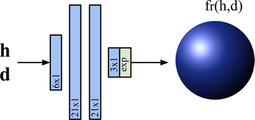
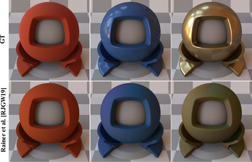
The parametrization of the network input strongly affects the reconstruction quality as it favours the learning of different aspects of the reflectance function. Rainer et al. [RJGW19] use a stereographic projection of the light and view directions in euclidean coordinates as network parameters. While this parametrization lends itself well to the modeling of effects like anisotropy, inter-shadowing and masking, which dominate the appearance of sparsely sampled spatially-varying materials, it is not well-suited to reconstruct specular highlights (as can be seen in Figure 2), which are much more noticeable in densely sampled uniform materials. In contrast, we use the Cartesian vectors  and
and  of the Rusinkiewicz parametrization [Rus98] for directions, which are a much better suited set of variables to encode specular lobes.
 (1)
(1)Conveniently, the architecture allows for unstructured sampling of the angular domain, allowing for a BRDF-aware adaptive random sampling of the upper hemisphere, for a total of  samples. We draw random uniform samples of the Rusinkiewicz parametrization angles, which emphasizes directions close to the specular highlight. In Section 4.1 we show that this is critical for accurate encoding of the specular highlights. The loss stabilises after 5 epochs for the more diffuse materials in Matusik et al.'s MERL database [MPBM03] (detailed in Section 3.4) while the most mirror-like ones can take up-to 90 epochs (between 10 seconds and 3 minutes on GPU).
NBRDF networks can be used to encode both isotropic and anisotropic materials. The latter introduce a further dependence on the Ruinskiewicz angle  , which must be learnt by the network. Following our sampling strategy, during training we draw random uniform samples from all four Rusinkiewicz angles, increasing the total number of samples five-fold to compensate for the increased complexity of the BRDF functional shape. In Section 4.2 we analyze the reconstruction of anisotropic materials from the RGL database [DJ18], which contains 51 isotropic and 11 anisotropic measured materials.
3.2 NBRDF autoencoder
Figure 3 shows our architecture for an autoencoder that learns a latent representation for NBRDFs. Input and output are the flattened weights of an NBRDF, which are further compressed by the network into short embeddings. In effect, the autoencoder learns to predict the weights of an NBRDF neural network. We typically use NBRDF encodings with two hidden layers  for a total of 675 parameters and encode them into embeddings of 32 values.
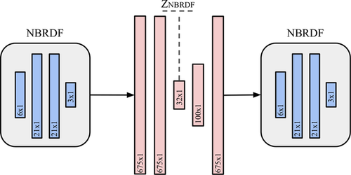
 , flattened to 1D vectors of 675 values.
In addition to further compressing the NBRDF representations, the autoencoder provides consistent encodings of the MERL materials that can be interpolated to generate new materials, as demonstrated in Section 4.3. Additionally, we show in Sections 3.3 and 4.4 that these consistent encodings can be used to predict parameters that can be leveraged for importance sampling.
Training of the autoencoder is performed using NBRDFs pre-trained with materials from MERL, employing a 80%-20% split between training and testing materials. To compensate for the limited availability of measured materials, we augment our data by applying all permutations of RGB channels for each material in the training set. The training loss used is image-based: our custom loss layer uses the predicted  vector to construct an NBRDF network of the original shape (
 ), and evaluates it to produce small renderings (
 ) of a sphere illuminated by a non-frontal directional light with
  , previously reported to produce more accurate results than headlight illumination on image-based BRDF fittings [SKWW19]. A fixed tone mapping (simple gamma curve with
  and low values bottom-clamped to
  ) is then applied to the sphere renderings, and the loss is computed as point-by-point MSE. The loss computation involves a differential implementation of the rendering pipeline for direct illumination and subsequent tone mapping, in order to keep the computation back-propagatable. Notably, applying a more traditional, non-image-based loss that attempts to match the input NBRDF weights fails to reconstruct the original appearances of the encoded materials.
3.3 Importance sampling
Importance sampling of BRDFs requires producing angular samples with a probability density function (PDF) approximately proportional to the BRDF. This can be accomplished by computing the inverse cumulative distribution function (inverse CDF) of the PDF, which constitutes a mapping between a uniform distribution and the target distribution. The computation of the inverse CDF of a PDF usually requires costly numerical integrations; however, for a set of parametric BRDF models, such as Blinn-Phong or GGX, this can be done analytically.
Our proposed method for quick inverse CDF computation is based on a shallow neural network, shown in Figure 4, that learns the mapping between the embeddings generated by the NBRDF autoencoder and a set of model parameters from an invertible analytic BRDF. In essence, the network learns to fit NBRDFs to an analytic model, an operation that is commonly performed through non-linear optimization, which is comparatively slow and prone to get lodged in local minima.

We use Blinn-Phong as target model for our prediction. Although it contains a total of seven model parameters, its associated PDF is monochrome and can be defined by only two parameters, associated with the roughness of the material and the relative weight between specular and diffuse components. Hence, we train our network to learn the mapping between the NBRDF's 32-value embeddings and the Blinn-Phong importance sampling parameters. Although the predicted PDF is an approximation of the original NBRDF, the resulting sampling is unbiased due to the exact correspondence between the sampling PDF and its inverse CDF, as shown in Section 4.4.
3.4 MERL Database
 ,
,  ) of the
  and
and  vectors from the Rusinkiewicz parametrization [Rus98]:
 : 90 samples from 0 to 90, with inverse square-root sampling that emphasises low angles.
 : 90 uniform samples from 0 to 90.
 : 180 uniform samples from 0 to 180. Values from 180 to 360 are computed by applying Helmholtz reciprocity.
Isotropic BRDFs are invariant in  , so the MERL database, which was created using a measurement setup relying on isotropic reflectance [MWL*99], omits
  . Counting all samples for the three colour channels, each material in MERL is encoded in tabular format with
  reflectance values (approx. 34 MB).
4 Results
In this section, we analyze our results on the reconstruction and importance sampling of measured materials. Although we centre most of our analysis on materials from the MERL database, we show that our approach can be applied to any source of measured BRDFs, as displayed in Figure 5. Reconstruction results for the complete set from MERL [MPBM03] and RGL [DJ18] databases can be found in the supplemental material. In addition, we have included our implementation of the NBRDF training in Keras [C*15], a Mitsuba plugin to render using our representation, and a dataset of pre-trained NBRDFs for materials from the MERL [MPBM03], RGL [DJ18] and Nielsen et al. [NJR15] databases.
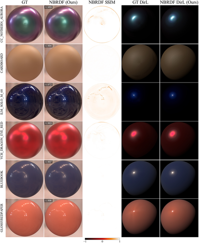
4.1 BRDF reconstruction
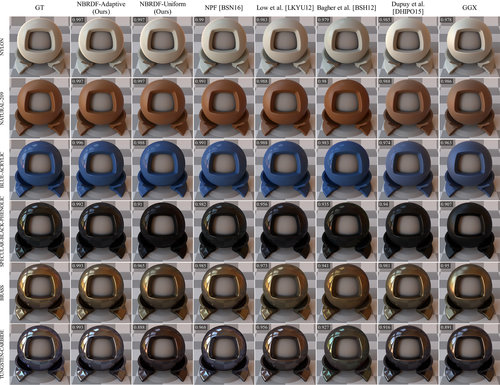
Figure 6 shows reconstruction performance on a visually diverse set of materials of the MERL database, for different approaches. We qualitatively compare the methods through renderings of a scene with environment map illumination. Ground truth is produced by interpolating the tabulated MERL data. The comparison reveals that most methods struggle with one particular type of materials: a GGX fit tends to blur the highlights, Bagher et al. [BSH12] on the other hand achieve accurate specular highlights, but the diffuse albedo seems too low overall. Out of all the proposed representations, our method produces the closest visual fits, followed by NPF [BSN16], a non-parametric BRDF fitting algorithm recently cited as state-of-the-art [DJ18]. As detailed in Section 2.1, a recent data-driven BRDF model by Dupuy and Jakob [DJ18] also compared favourably against NPF, although at an increased storage requirement.
 ).
).A quantitative analysis of the results, seen in Figure 7 and Table 1, shows that our representation outperforms the other methods in multiple image-based error metrics. In particular, NPF [BSN16] seems to lose fitting accuracy at very grazing angles, which is where the error is the highest on average (see Figure 7). A more detailed analysis of the functional shape of the NPF lobes confirms this observation. In Figure 8 we display polar plots (in log scale) of the specular lobes of two materials from MERL, comparing NBRDF and NPF fittings with ground truth for fixed incident angles. For low values of incident inclination  there is generally good agreement between all representations, while for grazing angles only NBRDFs are able to match the original shape. Furthermore, in the bottom plot we observe that NPF tends to produce unusually long tails. In the supplemental material we provide polar plot comparisons for the the full set of MERL materials.
| MAE | RMSE | SSIM | |
|---|---|---|---|
| NBRDF Adaptive Sampling | 0.0028  0.0034 0.0034 |
0.0033  0.0038 0.0038 |
0.995  0.008 0.008 |
| NBRDF Uniform Sampling | 0.0072  0.0129 0.0129 |
0.0078  0.0134 0.0134 |
0.984  0.029 0.029 |
| NPF [BSN16] | 0.0056  0.0046 0.0046 |
0.0062  0.0047 0.0047 |
0.990  0.008 0.008 |
| Low et al. [LKYU12] (ABC) | 0.0080  0.0070 0.0070 |
0.0088  0.0075 0.0075 |
0.986  0.012 0.012 |
| Bagher et al. [BSH12] (SGD) | 0.0157  0.0137 0.0137 |
0.0169  0.0145 0.0145 |
0.974  0.027 0.027 |
| Dupuy et al. [DHI*15] | 0.0174  0.0143 0.0143 |
0.0190  0.0151 0.0151 |
0.976  0.021 0.021 |
| GGX | 0.0189  0.0118 0.0118 |
0.0206  0.0126 0.0126 |
0.969  0.024 0.024 |

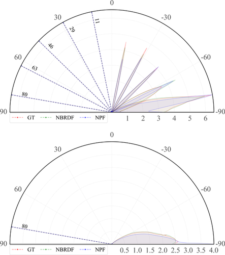
 . Top: grease-covered-steel. Bottom: black-oxidized-steel with a single fixed
  at
at  .
.One of the key components in successfully training the NBRDF networks is the angular sampling of the training loss. If training samples are concentrated near the specular lobe, the NBRDF will accurately reproduce the highlights. On the other hand, if the samples are regularly distributed, the Lambertian reflectance component will be captured more efficiently. We hence employ a BRDF-aware adaptive sampling of angles during training that emphasizes samples close to the reflectance lobes. In practice, we uniformly (randomly) sample the spherical angles of the Rusinkiewicz parametrization ( ,
,  and
and  ), which results in a sample concentration around the specular direction, while retaining sufficient coverage of the full hemisphere. Table 1 shows that this adaptive strategy for training sample generation produces much better results over the whole database and allows us to outperform analytic model fits in various error metrics.
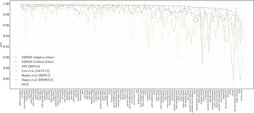
Finally, in Figure 10 we display the SSIM error for all materials from the MERL database, and for all discussed reconstruction methods. Our NBRDF adaptive-sampling outperforms other methods for almost all materials, with the exception of a small number of highly specular materials. Please refer to the supplemental material for a full detail of reconstructions, including all materials from the MERL and RGL [DJ18] databases.
4.2 Reconstruction of anisotropic materials
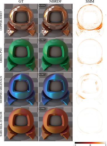
In Figure 9 we display the NBRDF reconstructions of multiple anisotropic materials from the RGL database [DJ18]. The networks used are the same as shown in the isotropic results of Figure 6 (i.e.  for a total of 675 weights). The reconstruction of the anisotropy is surprisingly robust, especially taking into account the compactness of the network size. There are, however, more perceivable differences in the visual fits than in the NBRDF isotropic encodings, which is reflected on the average SSIM error:
  . Lower reconstruction errors can be achieved by increasing the network size of the encoding NBRDF, providing great control over the level-of-detail of the representation. In Section 4.5 we will analyze the dependence of the reconstruction error with the network size, comparing with other representations in terms of memory footprint.
4.3 Latent space of materials
The generation of a unified encoding of the space of materials opens up many new possibilities. We use the NBRDF encodings of MERL materials to train our autoencoder that compresses NBRDFs to a 32-dimensional latent space.
In Table 2 we summarize various reconstruction error metrics comparing our autoencoding with PCA factorisation across MERL. Our implementation of PCA follows Nielsen et al.'s [NJR15], who proposed various improvements over traditional PCA, most importantly a log-mapping of reflectance values relative to a median BRDF measured over the training set. The training of both methods was performed with the same 80%-20% split of materials from MERL. The full set of renderings and errors can be found in the supplemental material.
| MAE | RMSE | SSIM | |
|---|---|---|---|
| NBRDF AE | 0.0178  0.013 0.013 |
0.0194  0.014 0.014 |
0.968  0.031 0.031 |
| PCA [NJR15] | 0.0199  0.008 0.008 |
0.0227  0.009 0.009 |
0.982  0.007 0.007 |
It is worth noting that the further reduction of NBRDFs from 675 parameters to 32 does not necessarily result in an effective compression of the representation in a practical use case, since the memory footprint of the decoder is roughly equivalent to 105 NBRDFs. In addition, preserving the maximum reconstruction quality requires storing the original NBRDF, since the autoencoder reduction inevitably leads to a degradation of the appearance after the decoding; however, this is not an issue as the main application of the autoencoder lies in the material embedding. Figure 11 shows a  -SNE clustering of the latent embedding learned by the autoencoder. The projection to the latent space behaves sensibly, as materials with similar albedo or shininess cluster together. This 32-dimensional encoding is the basis for our subsequent importance sampling parameter prediction.
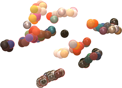
 -SNE clustering of MERL latent embeddings produced by the NBRDF autoencoder.Test set materials are indicated in red.
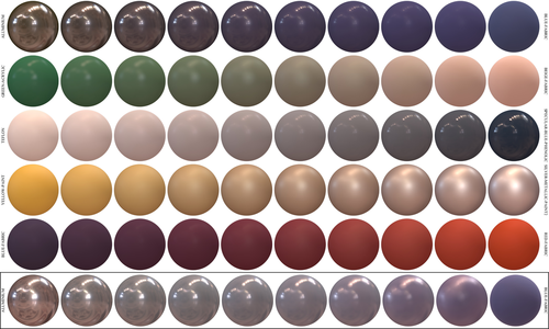
The stability of the latent space is further demonstrated in Figure 12, where we linearly interpolate, in latent space, between encodings of MERL materials, and visualize the resulting decoded materials. In contrast, the bottom row of Figure 12 shows the direct interpolation of the 675 parameters from two individually-trained NBRDF networks. Noticeably, this does not lead to a smooth transition of the specular properties of the two materials.
4.4 Importance sampling
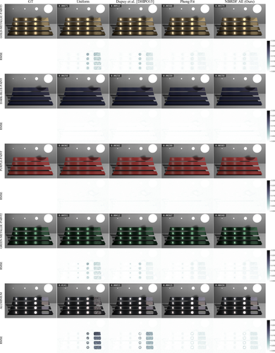
We leverage the stable embedding of materials provided by the autoencoder to predict importance sampling parameters. In practice, we train a network to predict the 2 Blinn-Phong distribution parameters that are used in the importance sampling routine. We train on a subset of materials from the MERL database, using fitted Blinn-Phong parameters from Ngan et al. [NDM05] as labels for supervised training. In Figure 13 we compare and analyze the effect of different importance sampling methods, applied to multiple materials from MERL unseen by our importance sampling prediction network. Renderings are produced with 64 samples per pixel, with the exception of the ground truth at 6400 spp. Each column is associated with a different importance sampling method, with all reflectance values begin evaluated from the original tabulated MERL data. We compare uniform sampling, Blinn-Phong distribution importance sampling (with optimized parameters, and predicted parameters from our network), and Dupuy et al.'s[DHI*15] routine. Even though a Blinn-Phong lobe is not expressive enough to accurately describe and fit the captured data, the parameters are sufficient to drive an efficient importance sampling of the reflectance distribution. Depending on the material, the predicted Blinn-Phong parameters can even reveal themselves better suited for importance sampling than the optimised Blinn-Phong parameters.
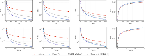
In addition to this image-based comparison, in Figure 14 we plot multiple error metrics as a function of samples per pixel, to compare the respective sampling methods. Both Phong and GGX-driven importance sampling converge quickly and keep a significant lead on uniform sampling. As shown in the plots, our importance sampling prediction can be tuned to GGX parameters (optimized labels from Bieron and Peers [BP20]) as well as to Blinn-Phong parameters, or any arbitrary distribution. For simplicity, we choose the Blinn-Phong distribution: more advanced models will provide a better reconstruction, but not necessarily provide a better sampling routine. More complex models might fit the specular lobe more precisely, but neglect other reflectance components of the data, such as sheen in fabric datasets for instance.

In Figure 15 we show importance sampling results for a complex scene. The majority of the original BRDFs in the scene have been replaced by materials from the MERL database, from the test set of our importance sampling parameter prediction network. We show crops from the renderings and compare our Phong-based importance sampling performance with uniform sampling and the method by Dupuy et al. [DHI*15]. Our method consistently shows lower noise in the scene, as also reflected in the numerical errors of Figure 16 which show a faster convergence for our method in terms of samples-per-pixel and render time.

4.5 Computational performance
We compare the performance of our combined pipeline (NBRDF reconstruction, with Phong-based importance sampling), to other compact representations that combine fast BRDF evaluation and built-in importance sampling strategies. All evaluations were performed with CPU implementations in Mitsuba, running on an Intel Core i9-9900K CPU. Table 3 shows that an unoptimized implementation of NBRDFs, combined with Phong importance sampling, although slower than other representations, offers comparable rendering performance, even to simple analytic models such as Cook-Torrance.
 )
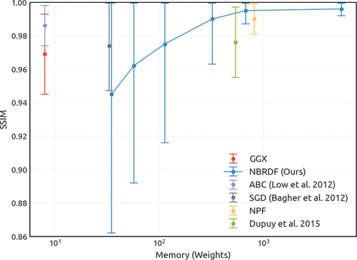
)Finally, in Figure 17 we compare multiple BRDF representation methods in terms of the average reconstruction SSIM error in the MERL database, and the memory footprint of the encoding. We show that the NBRDF network size can be adjusted to select the reconstruction accuracy. For very small networks ( weights) the NBRDF reconstruction is inaccurate, and thus parametric representations are to be preferred. However, for NBRDF networks of
  weights the reconstruction accuracy is already better than the best parametric encoding (Low et al. [LKYU12]) and equivalent to a state-of-the-art non-parametric method (NPF [BSN16]).
5 Conclusions
We propose a compact, accurate neural representation to encode real-world isotropic and anisotropic measured BRDFs. Combining the learning power of neural networks with a continuous parametrization allows us to train a representation that implicitly interpolates, and preserves fidelity to the original data at high compression rates. A new network instance is trained for every new material, but the training is fast and efficient as the networks are very light-weight.
We also show that the models are sufficiently well behaved to be further compressed by an autoencoder. The learned embedding space of materials open doors to new applications such as interpolating between materials, and learning to predict material-related properties. Specifically, we show that the latent positions can be mapped to importance sampling parameters of a given distribution. The computational cost of network evaluation is not significantly higher than equivalent analytic BRDFs, and the added importance sampling routine allows us to get comparable rendering convergence speed. Overall, our model provides a high-accuracy real-world BRDF representation, at a rendering performance comparable to analytic models.
In future work, our architecture could be applied to spatially-varying materials, for instance to derive spatially-varying importance sampling parameters on-the-fly, for procedurally created objects and materials. Similarly to the importance sampling parameter prediction, our meta-learning architecture can be used to learn further mappings, enabling applications such as perceptual material editing, and fast analytic model fitting.
Acknowledgements
This project has received funding from the European Union's Horizon 2020 research and innovation program under the Marie Skłodowska-Curie grant agreement no. 642841 (DISTRO ITN).


