Effects of ENSO on hydrological process and hydropower across the Lancang-Mekong River Basin
Abstract
Rapid growth in energy demand and accompanying hydropower development has been observed in the Lancang-Mekong River Basin (LMRB) in the last two decades. However, climate-induced variations in water resources have brought uncertainties and challenges to energy security across the LMRB, especially for the hydropower sector. In this study, we propose a multiscale approach by linking two spatially distributed models to simulate and evaluate the effects of climatic drivers both on the water resources and hydropower generations in the LMRB. Specifically, we evaluate the effects of midterm large-scale climatic drivers (i.e., ENSO) on the local hydrometeorological process and energy production. During ENSO events, the midstream to downstream LMRB is more impacted than the upstream LMRB, leading to hydroelectricity anomalies in the LMRB varying within a range of ±11,000 GWh. However, basin-wide drought conditions caused by El Niño events in the LMRB do not always result in a reduction in hydropower generation. The proposed approach provides a methodological basis for characterizing power system responses to climatic drivers, potentially informing the future energy strategy and infrastructure development in the LMRB.
1 INTRODUCTION
Rapid growth in the energy demand and accompanying hydropower development have been observed across the globe. In 2020, hydropower contributes a record 4418 TWh, remaining the largest renewable source of electricity (IEA, 2021a). The global installed hydropower capacity has continued to grow steadily in recent decades, reaching 1330 GW in 2020 (IHA, 2022). It is expected to continue growing in response to ongoing industrialization, economic development, and climate change. It is suggested that 2600 GW of hydropower capacity will be needed to reach net zero emissions by 2050 (IEA, 2021b).
However, hydropower and the entire energy system are also affected by climatic factors. The timing and magnitude of precipitation patterns may change and the evapotranspiration may increase due to rising temperatures, leading to the alteration in flow regimes (Cáceres et al., 2022). These meteorological factors could have compound effects on energy system, including effects on the demand side (Fan et al., 2019; van Vliet et al., 2012), effects on the supply side (Chandel et al., 2011; Su et al., 2017), spatial domains (Majone et al., 2016; Markoff & Cullen, 2008; Turner et al., 2017; Voisin et al., 2020), and adaption strategies (Eser et al., 2018; Szinai et al., 2020; Watcharejyothin & Shrestha, 2009). Moreover, multiple studies have revealed the regional heterogeneous relationship between climate and hydropower (B. Wang et al., 2014). Thus, it is imperative to evaluate the effects of climatic drivers on hydropower generation to examine the resilience of energy system, especially for regions relying on a large portion of hydropower, such as the Lancang-Mekong River Basin (LMRB).
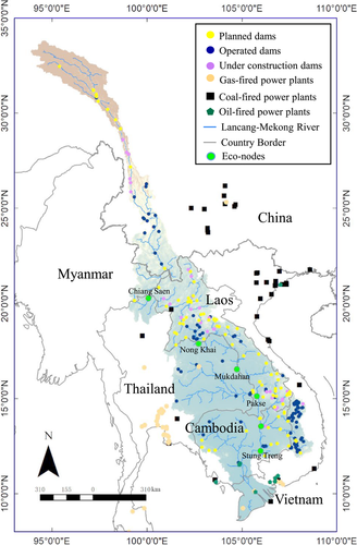
The Lancang-Mekong River is one of the largest and most controversial international rivers in the world, flowing across six riparian countries (i.e., China, Myanmar, Laos, Thailand, Cambodia, and Vietnam), as shown in Figure 1. The LMRB has an annual discharge of 475 km3 and covers an area of 795,000 km2, providing livelihood resources to approximately 64.8 million people (Mirumachi, 2020). The hydropower potential of the LMRB is approximately 268,000 GWh/year (Schmitt et al., 2019). The construction of large dams (dam height > 15 m) for hydropower and irrigation started in the 1960s and became more intensive after the late 1990s (Räsänen et al., 2018). In addition to the six hydropower dams built on the mainstream of the Lancang River by China with a total capacity of 15.6 GW (Han et al., 2019; Yu et al., 2019), 59 hydropower projects with a total installed capacity of 10,017 MW had been developed in the Mekong River basin, exploiting approximately 35% of the total estimated hydropower potential of that area (MRC, 2019). On the mainstream, 11 dams are proposed and being constructed with 9 in Laos and 2 in Cambodia (ICEM, 2009; MRC, 2010a), which could generate approximately 15,000 MW of hydropower and are projected to account for 8% of regional demand by 2025 (Grumbine & Xu, 2011). Growing dependency on hydropower may lead to more possibilities of power system loss or even failure under varying and changing climate conditions. Understanding the effects of climatic drivers on the power system, that is, the nexus among climate, water, and hydropower, is a key step toward a reliable and resilient power system in the LMRB.
ENSO is most likely the best-known climatic factor influencing hydrologic circulation and hydropower generation in the LMRB. ENSO is a coupled ocean–atmosphere phenomenon occurring in the tropical Pacific Ocean that affects oceans, climate, and hydrology at a global scale (Räsänen & Kummu, 2013; Ward et al., 2010). Its characteristic warming (El Niño) and cooling (La Niña) phases result in flood and drought conditions in many regions of the world, including the LMRB (Irannezhad et al., 2020; Y.-C. Liang et al., 2016; Räsänen et al., 2016; Ward et al., 2014). This ENSO-driven variation in water availability is certainly related to hydroelectric power production, but few studies have examined this hypothesis in detail (Chowdhury, Dang, Thai Nguyen, et al., 2020; Ng et al., 2017; Voisin et al., 2018). Ng et al. (2017) pointed out that although the positive and negative anomalies exist simultaneously and effectively cancel each other out at global and continental scales, the variabilities of hydropower production anomalies in specific regions induced by ENSO need to be treated with caution. Chowdhury, Dang, Thai Nguyen, et al. (2020) estimated that the anomalies of available hydropower in the Laotian–Thailand power system vary between ±4000 GWh due to ENSO. At the basin scale, the effects of ENSO on the LMRB's power system remain an interesting but challenging issue.
In this paper, we propose a multiscale approach by linking two spatially distributed models, that is, a hydrological model to simulate the relationship between hydrometeorological forces and water availability in the LMRB, and a power system planning and management optimization model to explicitly optimize the operating decisions made by the riparian countries. The research goals are threefold: (1) to simulate power sector development constrained by historical demand and natural hydrological status, aiming at both validating the proposed models and evaluating historical decisions on infrastructure development; (2) to illustrate the effects of ENSO on the local hydrometeorological process; (3) to examine how ENSO influences the hydropower sector security in the LMRB. The approach is demonstrated by taking the LMRB as a case. The rest of the paper is organized as follows. The methods are introduced first. Then, results are reported and followed by conclusion.
2 METHODOLOGY
2.1 Linked water and energy model
We develop a linked water and energy model to evaluate the effects of ENSO on water-energy nexus in the LMRB. Since Myanmar's contributions to streamflow (2%), basin population (<1%), basin area (3%), and energy demand/supply (~2%) are very low (Gao et al., 2021; Li et al., 2019; Ringler, 2001), it is not taken into consideration in this study. We employ a spatially distributed hydrological model (Coupled Routing and Excess Storage [CREST] model) as the water model to simulate the hydrologic response and water availability under different climate conditions in the LMRB (J. Wang et al., 2011). The energy model, which is energy system planning and management (ESPM) optimization model, is newly developed in this paper to analyze the LMRB's power sector. The variables, parameters, and their valid domains are presented in Nomenclature.
2.2 Water model
Since the available historical streamflow data (obtained from the MRC) are from gauge stations located on the mainstem of the rivers but streamflow records along the tributaries are unavailable, a water model is required to simulate a natural streamflow time series in the mainstem and tributaries of the LMRB. In our study, the CREST model (J. Wang et al., 2011) is employed to simulate the hydrologic response and water availability in the LMRB. CREST is a distributed hydrological model jointly developed by the University of Oklahoma and the National Aeronautics and Space Administration (NASA) SERVIR Project Team. CREST has been demonstrated to provide accurate streamflow simulations in the LMRB (Gao et al., 2021, 2022; Han et al., 2019; Li et al., 2019).
 ()
()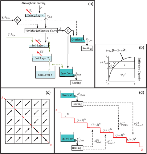
In Equation (1),  is the total cell water storage, including all water stored in the vegetation canopy, three soil layers, and the two linear reservoirs.
  is precipitation.
  is the actual evapotranspiration determined by both potential evapotranspiration (PET;
  ) and the vertically integrated water contents within one cell.
  and
and  denote the inflow generated from overland excess rain and interflow excess rain, respectively. A variable infiltration curve updated from the Xinanjiang model (Zhao, 1992) and the VIC model (X. Liang et al., 1996), is employed to separate precipitation into overland runoff and infiltration (see Figure 2b). The summations for interflow and overland flow in Equation (1) correspond to contributing runoff of multiple upstream cells.
  and
and  , which are passed to downstream routing, denote the outflow and generated from overland excess rain and interflow excess rain, respectively. Overland water movement and channel flow between the cells are based on flow direction and basin boundary derived from a digital elevation model (DEM) (see Figure 2c). Sub-grid cell routing, downstream routing, and subsurface runoff distribution from one cell to its downstream cells are illustrated in Figure 2d. The input data required to run CREST are: precipitation data (
 ), PET (
 ), and DEM.
2.3 ESPM optimization model
Although this study focuses on the effects of ENSO on hydropower generation in the LMRB, hydropower is not the only electricity source in the whole system. When water availability is affected in the LMRB, hydropower stations' generating capacity may be affected. From the perspective of economic reasons and for people's livelihood, instead of draining out the reservoirs and pushing the hydropower stations to their limits, the local governments may choose to put more alternative generation units as substitution of hydropower into operation as a precautionary measure (Siala et al., 2021; Sridharan et al., 2019). Meanwhile, regional interconnection may mitigate some of the climatic effects on hydropower (Cáceres et al., 2022). Therefore, the effects of ENSO on water resources and hydropower generation have to be evaluated in a framework where multi-sources of electricity are included.
The ESPM optimization model is newly developed to analyze the LMRB's power sector in this paper. The ESPM is a dynamic, bottom-up, multiyear energy system model. The ESPM produces an optimal power generation mix and decisions of hydropower plant generations, aiming at minimizing the cost of the whole power system in the planning horizon. It considers a technology portfolio inclusive of the LMRB's hydro, wind, solar PV, and fossil fuel-based power generation options. Existing, committed, and planned site-specific hydropower plants are included in the ESPM, covering 167 hydropower plants and maintaining their topology in the LMRB. Other generation options are represented using an aggregate total for their capacity in each riparian country following (Sridharan et al., 2019). In the ESPM, the riparian countries in the LMRB are linked using intercountry trade connectors that represent the cross-border electricity transmission networks in an integrated way.
 ) of year y. In each year, the power plants portfolio could either remain the same or be optimized, which means that ESPM could choose to bring new generating units into operation. If the portfolio is optimized in year y, it would be transferred to the next year (
 ). The costs can be divided into costs for investment in new generation units (
 ), fixed and maintenance costs (
 ), variable production costs (
 ).
).  includes the amortized construction costs (
 ) of new hydropower plants and the expansion costs of renewable generating units of type
  and thermal generating units of fuel
  ={coal, oil, gas} during the planning horizon. Typically, the larger the hydropower plant is, the lower the amortized construction costs. The amortized construction costs of the new built dams built in previous years are considered in
  .
.  consists of thermal power plants' startup costs (
 ), variable costs for heat rate (
 ) and fuel price (
 ) (Chowdhury et al., 2019). Therefore, the objective function is as Equations (2a-2d):
 ()
()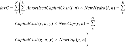 ()
()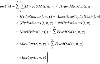 ()
()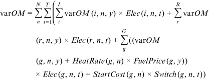 ()
() ,
,  , and
, and  are the power generation of the hydropower plant
  , renewable power plant of type
  , and thermal power plant of fuel
  in country
  during period
  , respectively. For hydropower plants,
  is a binary variable indicator describing the initial state of the ith hydropower plant in country
  . The model is forced to invest and bring in new hydropower plants and/or new power plants of other types to either meet the growing power demands or reduce the economic costs for generation.
  and
and  are binary variables denoting the construction status of the hydropower plant
  in country
  .
.Constraints considered in the ESPM include construction status, generating capacity, operational status, water balance, agricultural irrigation water withdrawal, minimum ecological release flow, and reservoir storage capacity.
2.3.1 Constraints related to hydropower plants
For hydropower plants, the ESPM considers the following constraints: water balance (Equations 3 and 4), agricultural irrigation water withdrawal ( in Equation 3), minimum ecological release flows (Equation 6,
  ) (Steffen et al., 2015), and reservoir storage capacity (Equation 7).
 is the release from all the nearest reservoirs that are located in the upstream of reservoir i in country n.
  is the lateral inflow.
  is the storage of reservoir i.
  ,
,  , and
, and  are the total release, spill release, and the release running over the turbine of hydropower plant i in country n.
 is a quadratic function of the reservoir's current storage
  , as stated in Equation (5).
 ()
() ()
() ()
() ()
() ()
()2.3.2 Thermal power plants operation
 and
and  are two decision variables describing the operational status (online or offline, to be started up or shut down, in %) of the thermal plant, and they are constrained by Equation (8):
 ()
()2.3.3 Power generation capacity
 the maximum capacity of the thermal power plant of fuel g in country n during year y;
  the maximum capacity of the type r renewable power plant in country n during year y;
  the maximum capacity of the hydropower plant i in country n.
 ()
() ()
() ()
() ()
()2.3.4 Energy balance
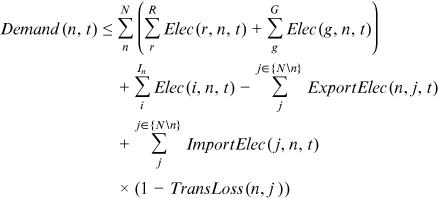
 ) connected to any other riparian country j in month t. The energy demand (
 ) can be matched through domestic power generation and the importation of electricity from neighboring countries, excluding the exported amount.
  is the export power from country
  to
to  in period t, and
  is the import power from country
  to
to  in period t. The transmission losses are taken into consideration. The transmission capacity between countries n and j is represented in Equations (11a-11b), where
  denotes the maximum capacity of the aggregated transmission line between the two countries.
 ()
() ()
() ()
()2.3.5 Hydropower plants status
 ()
() ()
() is the ith hydropower plant's status in country
  in year y and
  denotes whether to convert the ith hydropower plant's status from planned to committed.
2.3.6 Expansion of thermal and renewable power plants
 ()
() ()
()2.4 Model inputs
We applied the following data sets as inputs for the CREST model: the 3 hourly 0.1° gridded precipitation data from the latest version (V2.2) of the Multi-Source Weighted-Ensemble Precipitation (MSWEP) product (http://www.gloh2o.org/) (Beck et al., 2017), the PET data from the global daily data set provided by the Global Land Evaporation Amsterdam Model (GLEAM V3) (https://www.gleam.eu/), and the Global 30 arcsec Elevation (GTOPO30) DEM available at https://www.usgs.gov/centers/eros/science/ (USGS, 2018).
The input data of ESPM and their sources are categorized as follows:
(1) Monthly series of streamflow simulated by CREST and monthly water withdrawal data. They are acquired from the Food and Agriculture Organization (FAO) Aquastat database (FAO, 2022) and the countries' statistics yearbooks. (2) Parameters of the committed and planned hydropower plants, acquired from: the MRC dam database, Global Reservoir, and Dam Database, Lancang River Hydropower Inc., the ASEAN Centre for Energy (ACE), and relative literature (Lehner et al., 2011; Li et al., 2019; MRC, 2010a; 2010b; Räsänen et al., 2018; Team, 2019). (3) Economic costs parameters of the coal-, oil-, and gas-fired power plants in each riparian country, that is, the expansion costs, variable production costs, the fixed operation and maintenance costs, and startup costs. They are obtained from the literature (Weidner et al., 2014; Chowdhury et al., 2019; Chowdhury, Dang, Bagchi, et al., 2020; Chowdhury, Dang, Thai Nguyen, et al., 2020; Global Energy Observatory & KTH Royal Institute of Technology in Stockholm, Enipedia, World Resources Institute, 2018; Sridharan et al., 2019). (4) Technology efficiency parameters of the coal-, oil-, and gas-fired power plants are calibrated during the historical period 2001–2005 with the value range obtained from the literature (Chowdhury et al., 2019; Chowdhury, Dang, Bagchi, et al., 2020; Chowdhury, Dang, Thai Nguyen, et al., 2020; Global Energy Observatory & KTH Royal Institute of Technology in Stockholm, Enipedia, World Resources Institute, 2018; Sridharan et al., 2019). (5) Parameters of the transmission lines, obtained through various reports (ADB, 2012; ECA, 2010). (6) Monthly time series of the riparian countries' power demands, limited to those in the LMRB. This is calculated by first combining each country's annual basin population, annual GDP per capita, and annual power consumption per capita to obtain the annual demand, and then disaggregated to monthly resolution using the monthly demand curve from previous studies (Chowdhury, Dang, Thai Nguyen, et al., 2020; Sridharan et al., 2019). This approach indicates that we assume that the power demand of each country in the LMRB resembles that of the whole country. (7) Statistical and forecasted annual prices of fossil fuels, obtained from Sridharan et al. (2019). (8) Technology cost assumptions for solar PV, wind onshore power plants are in consistent with Siala et al. (2021).
2.5 Experimental setup and analysis
First, we validate our model framework in the historical period. We use the available historical streamflow observation during 1980–2014 to calibrate and validate the CREST model, and the simulated streamflow sequences across the LMRB are passed to the ESPM. Due to data availability, the ESPM is validated against 2001–2005 data on generation mix and data on cross-border electricity trade in the year 2016. Second, to understand how ENSO affects the LMRB's power system performance, we keep the power plants, transmission facilities, and power demand the same as the actual conditions in 2016, while the CREST is forced with 37 years of precipitation and PET data spanning the period 1980–2016. In other words, the exposure of the status quo power system to hydro-climatic variations observed in recent years is evaluated.
The standardized streamflow index (SSI) is applied to evaluate the hydrological extremes and impact of climate change. The SSI index is calculated through the following steps. Following Vicente-Serrano et al. (2012), we use probability distributions to fit the monthly streamflow series and then normalize them to obtain the SSI at different eco-nodes, as shown in Figure 1. The SSIs are averaged to produce one index for the LMRB. To consider the ENSO impacts, each year is classified as either Neutral, El Niño, or La Niña (as shown in Table 1), according to the Japan Meteorological Agency (https://www.coaps.fsu.edu/jma) and Chowdhury, Dang, Thai Nguyen, et al. (2020). The bimonthly Multivariate El Niño/Southern Oscillation (ENSO) index (MEI.v2) (https://psl.noaa.gov/enso/mei/) is employed to conduct the correlation analysis and explore the relationship between ENSO and the LMRB's hydrological processes, using the precipitation and evapotranspiration data over the period of 1980–2016. MEI.v2 is calculated from the leading combined empirical orthogonal function of five different variables (sea level pressure, sea surface temperature, zonal and meridional components of the surface wind, and outgoing longwave radiation) over the tropical Pacific basin (30°S–30°N and 100°E–70°W). The January–February–March (JFM) forms part of the peaking period of ENSO events, and the MEI index values from these months (MEIJFM) represent the occurrence and strength of individual ENSO events.
| ENSO phase | Years |
|---|---|
| El Niño (warm phase) | 1983, 1987, 1992, 1998, 2003, 2007, 2010, 2015, 2016 |
| Neutral | 1980–1982, 1984, 1986, 1990, 1993–1997, 2001, 2002, 2004–2006, 2009, 2012–2014 |
| La Niña (cold phase) | 1989, 1999, 2000, 2008, 2011 |
- Abbreviation: ENSO, El Niño/Southern Oscillation.
3 RESULTS
3.1 Model performance
 ()
() ()
() ()
() is the observed streamflow; and
  is the simulated streamflow. The periods between 1980–1987, 1988–2007, and 2008–2014 were defined as the model calibration period, validation period, and impact period, respectively. The results are shown in Table 2.
During the calibration period, there were almost no reservoirs constructed in the basin whilst during validation period 1, several small reservoirs were constructed (Yu et al., 2019). The two large reservoirs with seasonal regulation capacity, Xiaowan and Nuozhadu reservoirs, were built on the mainstem during validation period 2, resulting in changes to the downstream flow regime (Li et al., 2017). In general, CREST provides satisfactory performance in simulating natural streamflow with the NSE ranges of 0.83–0.93, 0.85–0.93, and 0.42–0.90 during calibration, validation, and impact periods, respectively. The difference between the simulated streamflow and observed streamflow regimes was greater in the upstream region. This difference in impact period was mainly attributed to the impact of China's dam construction and operation. As such, using simulated natural flow was better than using the observed streamflow as reservoir operations have altered the natural streamflow.
 ) and the statistical data (
 ) from the world bank database and China's statistical yearbook. Since the statistical data of Laos is missing, we only evaluate the results of the rest four countries.
 ()
()| Gauging stations | NSE | CC | Bias (%) | ||||||
|---|---|---|---|---|---|---|---|---|---|
| Calibration | Validation | Impact | Calibration | Validation | Impact | Calibration | Validation | Impact | |
| Chiang Saen | 0.83 | 0.85 | 0.42 | 0.95 | 0.93 | 0.84 | −1.53 | −6.05 | −4.70 |
| Nong Khai | 0.93 | 0.90 | 0.60 | 0.97 | 0.95 | 0.84 | −4.05 | −4.55 | −0.69 |
| Mukdahan | 0.93 | 0.93 | 0.88 | 0.94 | 0.96 | 0.95 | −7.21 | −11.93 | −15.74 |
| Pakse | 0.92 | 0.93 | 0.90 | 0.96 | 0.97 | 0.97 | −0.08 | −1.25 | 0.45 |
| Stung Treng | 0.92 | 0.90 | 0.84 | 0.96 | 0.95 | 0.97 | 12.19 | 2.47 | 12.73 |
- Abbreviations: CC, correlation coefficient; NSE, Nash–Sutcliffe efficiency.
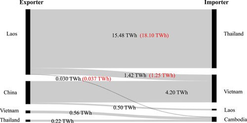
The performance metrics of ESPM are presented in Table 3. ESPM provides satisfactory performance in simulating electricity generation mix. The ESPM results of cross-border electricity trade based on the transmission infrastructure state in 2016 are compared with the available statistics, shown in Figure 3. The numbers in black and red are ESPM outputs and statistical data, respectively. Our model captures the patterns of electricity trading among the countries, where Laos and China are the main exporters, while Thailand and Vietnam are the main importers. These results together suggest that our model could be used for further analysis.
| Country | Electricity category | RMSE | Country | Electricity category | RMSE |
|---|---|---|---|---|---|
| China | Hydro | 8.73 | Cambodia | Hydro | 3.93 |
| Coal | 8.74 | Coal | 0.00 | ||
| Oil | 0.00 | Oil | 4.95 | ||
| Gas | 0.06 | Gas | 0.00 | ||
| Renewable excludes hydro | 0.00 | Renewable excludes hydro | 1.14 | ||
| Thailand | Hydro | 1.47 | Vietnam | Hydro | 7.25 |
| Coal | 6.79 | Coal | 3.66 | ||
| Oil | 3.48 | Oil | 3.71 | ||
| Gas | 7.08 | Gas | 4.22 | ||
| Renewable excludes hydro | 0.89 | Renewable excludes hydro | 0.04 |
- Abbreviations: ESPM, energy system planning and management; RMSE, root mean squared error.
3.2 Effects of ENSO on the hydrological process in the LMRB
Figure 4a presents the relationship between the annual mean values of SSI and annual precipitation in the LMRB. El Niño is closely related to droughts in the LMRB (negative values of SSI), while La Niña usually implies a wet year (positive values of SSI). However, two exceptions are found. One is the 1989 La Niña, when positive rainfall anomalies were confined to central Vietnam, while the remaining areas were drier than average (Chowdhury, Dang, Thai Nguyen, et al., 2020; Räsänen et al., 2016). Another is the 2016 El Niño, which actually developed in 2015 and lasted until 2016. Although it was recorded to be one of the strongest El Niño events, causing various degrees of droughts from January to May in the LMRB and leading to emergency water supplementation from the Lancang River in China (MRC, 2016), the annual mean SSI at the basin scale was balanced by wet conditions both in upstream and during the wet season (see Figure 4b,c). It is notable that the water availability conditions across the LMRB are not always synchronous. Figure 4b,c shows the SSI time series at Chiang Saen station (upstream) and Stung Treng station (downstream), respectively. We can see that the magnitudes and durations of the droughts (shown in red bars) at these two stations do not always match. This is related to the temporal and spatial effects of ENSO.

 ) are shown in red bars. The El Niño and La Niña years are shadowed in light yellow and blue, respectively.
To illustrate the temporal and spatial effects of ENSO, the general evolution of ENSO-related precipitation and PET patterns needs to be analyzed. Here we use the precipitation and PET data over the period 1980–2016 to explore the general pattern of ENSO's effect on the LMRB.
Previous studies have indicated that ENSO events are generally 2-year phenomena, starting in spring, maturing late in the same year or early the next year, and decaying in the following summer (Räsänen et al., 2016). Therefore, precipitation and PET are aggregated into seasonal sums, that is, December–January–February in the first year (DJF(0/1), March–April–May in the second year (MAM(1)), June–July–August in the second year (JJA(1)), and September–October–November in the second year (SON(1)). The notations “0” and “1” in the names of the seasons denote the first year (i.e., developing year) and the second year (i.e., decaying year) of an ENSO event, respectively. The precipitation and PET are correlated with the time series of MEIJFM at the grid level, resulting in seasonal correlation maps. These results are provided in Figure 5, where the first and second rows are correlation maps of MEIJFM with PET and precipitation, respectively. The black arrow indicates the chronological order. The negative (positive) correlation between MEIJFM and precipitation (PET) indicates reduced precipitation (increased PET) during El Niño and increased precipitation (decreased PET) during La Niña, leading to dry conditions in El Niño and wet conditions in La Niña.
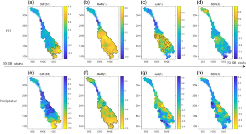
As ENSO events gradually mature from DJF(0/1) to MAM(1), in a large fraction of the midstream area, that is, Laos, eastern Thailand, and Cambodia, the correlation between MEIJFM and precipitation (PET) converts from a positive (negative) correlation to a negative (positive) correlation. The Mekong Delta in Vietnam first exhibits a strong negative (positive) correlation between MEIJFM and precipitation (PET) in DJF(0/1), implying that the Mekong Delta is more likely to be subjected to severe droughts during El Niño events. This is confirmed by Räsänen et al. (2016), in which the March-May precipitation anomalies for eight El Niño events were calculated. Although the precipitation anomaly patterns vary between different events, but negative precipitation anomalies widely spread in the LMRB, and the Mekong Delta frequently encounters droughts, such as in the El Niño event of 1997–1998.
When moving from MAM(1) to SON(1), the negative (positive) correlation between MEIJFM and precipitation (PET) disappears gradually. However, the MEIJFM and precipitation (or PET) in the middle reaches of the upstream Lancang River in China do not present correlations throughout the ENSO process. Furthermore, the source area of the upstream Lancang River located on the Tibetan Plateau in China exhibits negative correlations between MEIJFM and precipitation in MAM(1), without an observable significant correlation between MEIJFM and PET during ENSO. This indicates that the Lancang River part is less impacted by ENSO than the midstream to downstream LMRB.
3.3 Effects of ENSO on the LMRB's power system
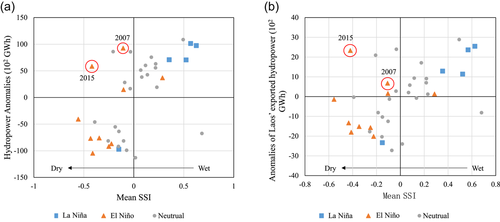
The effects of ENSO on hydropower generation in the LMRB are shown in Figure 6. Hydropower production generally reveals a positive correlation with the mean SSI, which is in accordance with previous studies (Gao et al., 2021). The anomalies of hydroelectricity in the LMRB vary by up to ±11,000 GWh, larger than the ±4000 GWh estimated by Chowdhury, Dang, Thai Nguyen, et al. (2020). This is because Chowdhury, Dang, Thai Nguyen, et al. (2020) included only the hydropower generation in the Laotian–Thailand subbasin, while we consider the whole LMRB, including the upstream part in China, with many large hydropower plants. Although China's dams have a larger storage capacity than the downstream dams, they do not have an interannual regulating ability to smooth interannual climatic variations. Moreover, irrigation water withdrawals are satisfied before hydropower generation in the ESPM; thus fluctuations in hydropower generation are inevitable. These fluctuations are also found in Laos' exported hydropower generation (shown in Figure 6b), which varies by ±2800 GWh. Laos represents the second-largest hydropower generator and the largest exporter in the LMRB, with approximately two thirds of its hydroelectricity production exported (IHA, 2016). Thus, the anomalies of Laos' exported hydroelectricity vary with the anomalies of the LMRB's total hydropower generation.
As the hydropower generation in the LMRB fluctuates with the water resources availability and the electricity demand from the society must be met (see Equation 10), more thermal generating units would be forced into operation, as the installed capacity of renewable energy such as solar PV and wind is limited. This would in return leads to a higher emission of CO2 and higher generation cost of the energy system. Moreover, previous studies have pointed out that droughts could affect local freshwater-dependent electric plants (Byers et al., 2020). Chowdhury, Dang, Thai Nguyen, et al. (2020) found that during El Niño the largest value of derated capacity of thermoelectric plants is ~1500 MW in Thailand and ~750 MW in Laos, which corresponds to about 27% and 40% of the installed capacity. In case where a large portion of the electric plants are freshwater-dependent, the ENSO's effect on the energy system could be magnified. Since in this study the focus falls on the hydropower in the LMRB, other generation options in the ESPM are represented in an aggregate way, making it difficult to quantify the ENSO's effects on other electricity sources considering the heterogeneity of the ENSO's spatial pattern and effect on the water resources. But the vulnerabilities in hydropower and thermoelectricity could be turned into opportunities for developing renewable energies, which are less dependent on the water resources and also more environmentally friendly.
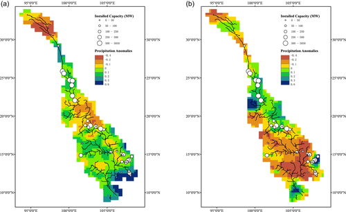
However, basin-wide drought conditions or El Niño events in the LMRB do not always result in a reduction in hydropower generation. Two special years, that is, 2007 and 2015, are marked in Figure 6 and detailed in Figure 7. In these 2 years, although El Niño events are observed and the LMRB experiences droughts (negative values of mean SSI), the total hydropower generation of the LMRB and Laos' exported hydroelectricity do not exhibit negative anomalies. This phenomenon can be explained by Figure 7, which shows the spatial distributions of precipitation anomalies in 2007 (Figure 7a) and 2015 (Figure 7b). Although the LMRB receives reduced precipitation in these 2 years at the basin level, different spatial distribution patterns are observed. In 2007, the largest rainfall reduction occurs in the source region in China and the midstream region in Thailand, southern Laos, and Cambodia. However, in the middle reaches of the Lancang River in China, the Se Kong, Se San, and Sre Pok basins (known as the 3S-basin) exhibit positive precipitation anomalies. As shown in Figure 7a, these relatively wet regions also feature large hydropower plants (owned by China, Laos, and Vietnam). This indicates that although El Niño and basin-wide droughts occur in 2007, a major proportion of the LMRB's hydropower generating units are not exposed to droughts but become wetter than normal. Similar reasons can be used to explain 2015 in Figure 7b as well. However, there is a small difference in northern Laos, where large dams are located. Unlike in 2007, increased rainfall appears in this region, enabling Laos to produce more hydroelectricity. This leads to a larger positive anomaly in Laos' exported electricity than in 2007.
In conclusion, ENSO's effects on the hydroclimatic and streamflow conditions in the LMRB are profound, especially for the midstream to downstream region. During March–April–May of the year when the ENSO events decay, ENSO's effects on both the precipitation and PET are strongest and most consistent spatially. The hydropower production in the LMRB shows a positive relationship with the water availability conditions, with many negative anomalies of hydropower occurring in El Niño years. However, there are exceptions. The spatial pattern of precipitation anomalies during El Niño events is crucial, as it varies between individual El Niño events, causing different magnitudes of hydropower plant exposure to droughts and resulting in different hydropower reductions.
4 CONCLUSION
In this study, we propose a multiscale approach by linking a spatially distributed hydrological model CREST and a spatially distributed node-linked power system optimization model ESPM. The proposed approach can simulate and assess the effects of climatic and economic drivers on power development strategies. The approach is applied to evaluate the effect of ENSO on the power systems in the LMRB.
Our results show that ENSO's effects on the hydroclimatic and streamflow conditions in the LMRB are profound, but the water availability conditions across the LMRB are not always synchronous during ENSO events. The upstream Lancang River is less impacted by ENSO than the midstream and downstream LMRB. The anomalies of hydroelectricity in the LMRB vary with hydroclimatic variability in the range of ±11,000 GWh, which is significantly larger than previous estimates. However, our results indicate that the hydropower system's response to ENSO is determined not only on their severity, but also on their spatial footprint. Basin-wide drought conditions or El Niño events in the LMRB do not always result in a reduction in hydropower generation. Conclusions regarding certain facilities' resilience to the hydro-climatic variability should be treated with caution.
This study has certain limitations. We do not consider the cost of CO2 emissions, which may lead to a higher preference for hydropower and other renewable generating options. Moreover, our analysis is based on the current power system configuration. In reality, a number of new power plants and international trading programs are on the way. This could help relieve the pressure of the current system under extreme climatic events. In future studies, since the ESPM are capable of describing the evolution of the power system, the coupled effects of climatic events and infrastructure development in the LMRB's power system could be examined. By adding some parameters describing tax and subsidy policies, the influence of economic and social development on the electricity demand, the proposed approach could assess the effects of economic drivers on the power system development as well. Nevertheless, the proposed approach provides a methodological basis for characterizing the power system responses to multiple factors at the basin level. These limitations can be resolved in future work by introducing more factors to the proposed approach.
5 DISCLAIMER
Any statements expressed in these materials are those of the individual authors and do not necessarily represent the views of ASCE, which takes no responsibility for any statement made herein. No reference made in this publication to any specific method, product, process, or service constitutes or implies an endorsement, recommendation, or warranty thereof by ASCE. The materials are for general information only and do not represent a standard of ASCE, nor are they intended as a reference in purchase specifications, contracts, regulations, statutes, or any other legal document. ASCE makes no representation or warranty of any kind, whether expressed or implied, concerning the accuracy, completeness, suitability, or utility of any information, apparatus, product, or process discussed in this publication, and assumes no liability therefor. This information should not be used without first securing competent advice with respect to its suitability for any general or specific application. Anyone utilizing this information assumes all liability arising from such use, including but not limited to infringement of any patent or patents.
NOMENCLATURE
Coupled routing and excess storage (CREST) model
-

-
- total cell water storage, including all water stored in the vegetation canopy, three soil layers, and two linear reservoirs (mm)
-

-
- precipitation (mm/d)
-

-
- actual evapotranspiration determined by the potential evapotranspiration and vertically integrated water contents of a cell (mm/d)
-

-
- inflow generated from overland excess rain (mm/d)
-

-
- outflow generated from overland excess rain (mm/d)
-

-
- inflow generated from interflow excess rain (mm/d)
-

-
- outflow generated from interflow excess rain (mm/d)
Energy system planning and management optimization model (ESPM)
Indexes and sets
-

-
- time periods (years)
-

-
- time periods (months)
-

-
- hydropower plants
-

-
- countries (CHN, LAO, THA, KHM, and VNM)
-

-
- fuel types for thermal power plants (coal, oil, and gas)
-

-
- types of renewable power plants (solar and wind)
-

-
- set of months in one year
-

-
- set of countries (CHN, LAO, THA, KHM, and VNM)
-

-
- sets of hydropower plants in country

- sets of hydropower plants in country
-

-
- sets of hydropower plants that are located in the nearest upstream region of the hydropower plant

- sets of hydropower plants that are located in the nearest upstream region of the hydropower plant
-

-
- sets of thermal power plant fuels (coal, oil, and gas)
-

-
- sets of renewable power plant types (solar and wind)
Parameters
-

-
- capacity factor for renewable power plant of type
 in country
  during period
  (in %,
  )
) - capacity factor for renewable power plant of type
-

-
- agricultural irrigation water withdrawal in the river zone located downstream hydropower plant
 during period
  (Mm3)
(Mm3) - agricultural irrigation water withdrawal in the river zone located downstream hydropower plant
-

-
- lateral inflow for hydropower plant
 during period
  (km3)
(km3) - lateral inflow for hydropower plant
-

-
- minimum ecological release flows at hydropower plant
 during period
  (m3/s)
 - minimum ecological release flows at hydropower plant
-

-
- time duration of period
 (hour, h)
 - time duration of period
-

-
- price of fuel
 in year
  ($/MMBtu)
 - price of fuel
-

-
- power demand of country
 in period
  (MW h)
 - power demand of country
-

-
- the maximum capacity of the hydropower plants
 in country
  (MW)
(MW) - the maximum capacity of the hydropower plants
-

-
- generating efficiency of hydropower plant
 in country
  (in %,
  )
) - generating efficiency of hydropower plant
-

-
- amortized construction costs of new hydropower plant
 ($/MW)
 - amortized construction costs of new hydropower plant
-

-
- expansion costs of renewable power plant of type
 in country
  during year
  ($/MW)
 - expansion costs of renewable power plant of type
-

-
- expansion costs of thermal power plant of fuel
 in country
  during year
  ($/MW)
 - expansion costs of thermal power plant of fuel
-

-
- fixed and maintenance costs of hydropower plant
 in country
  during year
  ($/MW)
 - fixed and maintenance costs of hydropower plant
-

-
- fixed and maintenance costs of renewable power plant of type
 in country
  during year
  ($/MW)
 - fixed and maintenance costs of renewable power plant of type
-

-
- fixed and maintenance costs of thermal power plant of fuel
 in country
  during year
  ($/MW)
 - fixed and maintenance costs of thermal power plant of fuel
-

-
- variable production costs of hydropower plant
 in country
  during year
  ($/MW h)
 - variable production costs of hydropower plant
-

-
- variable production costs of renewable power plant of type
 in country
  during year
  ($/MW h)
 - variable production costs of renewable power plant of type
-

-
- variable production costs of thermal power plant of fuel
 in country
  during year
  ($/MW h)
 - variable production costs of thermal power plant of fuel
-

-
- variable costs for heat rate of thermal power plant of fuel
 in country
  (MMBtu/MW h)
 - variable costs for heat rate of thermal power plant of fuel
-

-
- start-up costs of thermal power plant
 ($/MW h)
 - start-up costs of thermal power plant
-

-
- transmission loss rate from country
 to country
  (%)
(%) - transmission loss rate from country
-

-
- maximum capacity of transmission lines between country
 and
and  (MW)
(MW) - maximum capacity of transmission lines between country
-

-
- dead storage of hydropower plant
 (Mm3)
(Mm3) - dead storage of hydropower plant
-

-
- total storage of hydropower plant
 (Mm3)
(Mm3) - total storage of hydropower plant
Nonnegative continuous variables
-

-
- newly added installed capacity of the
 th renewable power plant (MW)
 - newly added installed capacity of the
-

-
- newly added installed capacity of the
 th thermal power plant (MW)
 - newly added installed capacity of the
-

-
- maximum capacity of the renewable power plant type
 in country
  during year
  (MW)
(MW) - maximum capacity of the renewable power plant type
-

-
- maximum capacity of country n's the thermal power plant of fuel
 in country
  (MW)
(MW) - maximum capacity of country n's the thermal power plant of fuel
-

-
- variables describing the operational status (online or offline) of the country
 's thermal plant of fuel
  in period
  (%,
(%,  )
) - variables describing the operational status (online or offline) of the country
-

-
- variables describing the operational status (to be started up or shut down) of the
 th thermal plant (%,
  )
) - variables describing the operational status (to be started up or shut down) of the
-

-
- storage of hydropower plant
 in country
  during period
  (Mm3)
(Mm3) - storage of hydropower plant
-

-
- total release of hydropower plant
 in country
  during period
  (m3/s)
 - total release of hydropower plant
-

-
- spill release of hydropower plant
 (m3/s)
 - spill release of hydropower plant
-

-
- release running through the turbine of hydropower plant
 (m3/s)
 - release running through the turbine of hydropower plant
-

-
- hydraulic head of hydropower plant
 in country
  during period
  (m)
(m) - hydraulic head of hydropower plant
-

-
- power generation of hydropower plant
 in country
  during period
  (MW h)
 - power generation of hydropower plant
-

-
- power generation of renewable power plant
 in country
  during period
  (MW h)
 - power generation of renewable power plant
-

-
- power generation of thermal power plant
 in country
  during period
  (MW h)
 - power generation of thermal power plant
-

-
- export power from country
 to
to  in period
  (MW h)
 - export power from country
-

-
- import power from country
 to
to  in period
  (MW h)
 - import power from country
Binary variables
-

-
- equal to 1 if hydropower plant
 in country
  is built during year y and 0 otherwise
 - equal to 1 if hydropower plant
-

-
- equal to 1 if hydropower plant
 in country
  already exists during year y and 0 otherwise
 - equal to 1 if hydropower plant
-

-
- equal to 1 if hydropower plant
 in country
  already exists at the beginning of the whole optimization horizon and 0 otherwise
 - equal to 1 if hydropower plant
ACKNOWLEDGMENTS
This research was funded by the National Natural Science Foundation of China (92047302 and U2243215). The authors are grateful to the editors and the two anonymous reviewers for their constructive suggestions, which led to major improvements in the paper.
ETHICS STATEMENT
None declared.
Open Research
DATA AVAILABILITY STATEMENT
All data, models, and code generated or used during the study appear in the submitted article.


