2.1 Sequence and structural analysis of anti-spike antibodies

In this section, we analyze the peculiar traits characterizing anti-S protein antibodies.

Starting from the very first phases of the pandemic, the interaction between Spike and antibodies has been studied. In this work,⁵¹ polyclonal immunoglobulins from COVID-19 convalescent individuals have been characterized, providing some preliminary considerations regarding the antibodies side of the interface. Thus, the effort of the scientific community has been mainly focused on the description of the most immunogenic regions of the Spike protein, and how the variant's amino acid substitutions can impact the binding with known antibodies.^52-55 A complete overview of the various antibody-spike complexes experimentally determined has been furnished in this recent paper, with particular attention to the epitope region the antibodies are bound to.⁵⁶

However, we focused on a different aspect. We study antibody sequences (using the Chotia numbering scheme^{10, 11}), the number of residues composing CDRs, and the position of the antigen-contacting residues. To highlight eventual originalities, we select two distinct structural datasets composed of experimental structures of antibody–antigen complexes: in the Spike dataset, 298 antibody-S complexes are present while in the General dataset, we gather 684 antibody–antigen structures, to work as a control.

The results of these analyses are shown in Figure 1.

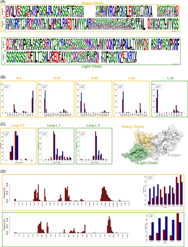
First, we investigate if the sequences of anti-Spike antibodies are statistically different with respect to the control sequences (antibodies binding proteins different from SARS-CoV-2 Spike). In particular, Figure 1. A shows the logo representations of both the heavy and the light antibodies chain belonging to the Spike dataset, obtained with a multiple sequence alignment and the WebLogo application.⁵⁷ For each residue in the antibody sequence, the probability to find the indicated amino acid in that position is indicated by the height of the corresponding letter. In Figure 1B, we report the positions where the differences with the control case are more evident. In particular, focusing on the positions populated almost in 75% of the antibodies (both in the Spike dataset and in the General dataset) we select the cases where it occurs a 25% difference in an amino acid frequency between the two datasets. It turns out that some important differences exist in positions H5, H40, H60, H83, and L43: compared to the control case, the anti-S antibodies use with more probability ALA in H40, H60, and L43 while they prefer VAL and ARG in H5 and H83, respectively.

Next, we focus our attention on the length of antibodies CDRs. For each of the six loops, we build the histogram regarding the number of residues composing the loop, using separately the Spike dataset and the General dataset. We thus compare the loop length distributions using the Kolmogorov–Smirnov statistical test. We report in Figure 1C the loops that result to be different (p-value $<$ .01): it can be noted that anti-spike antibodies typically employ an H2 CDR shorter than the control, while both L1 and L3 are characterized by a higher number of residues.

Lastly, we identify the antibody residues that are more involved in the interaction with the antigen (intuitively, in the Spike dataset the antigen is always the S protein). In our approach, an antibody residue is in contact with the antigen if its CA atom is closer than 8 Å to any antigen CA atom. In Figure 1D, we report the result of this analysis. In the left bar plots, we report the probability of antigen interaction regarding each antibody position, as obtained using the Spike dataset. As expected, both for heavy (upper panel) and light (lower panel) chains, the interaction with the antigen is mediated by the CDRs, as three well-separated peaks emerge from the plot. Interestingly, in the right panels, we show the comparison between the results in the Spike dataset and the General dataset: the residues with the most marked differences are reported in the upper and the lower panel for heavy and light chains, respectively. It has to be noted that anti-S protein antibodies use H1 residues to contact the antigen with more frequency than in the control case, while H3 is less preferred. Analogously, the interaction involving L1 residues is more common in anti-S antibodies than in the general case.

2.2 Preferential epitopes and energy of spike-antibodies interaction

Here, we focus our attention on the S protein side of the complexes, investigating where the S regions most prone to antibody binding are located and which the energetic mechanisms for the recognition are. Working on the Spike dataset, we define the intermolecular contact as in the previous section (i.e., an S residue is in contact with the antibody if its CA atom is closer than 8 Åto any CA of the antibody). Figure 2A shows the interaction frequency computed for each residue considering all the complexes in the dataset. The bars in yellow regard residues from the S NTD, whereas the bars in cyan refer to the ones in the RBD: among these residues, we depict in blue the ones involved in ACE2 recognition. This frequency determines the residue immunogenicity index, represented in Figure 2B, where the higher the red intensity, the higher the residue immunogenicity.

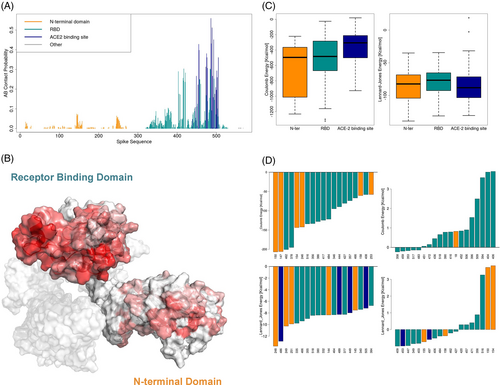
These results allow us to classify the antibody-Spike complexes in three categories, according to the S region used for the recognition: N-ter (27 complexes, 9% of the dataset), RBD (antibodies bound to RBD but not in the ACE2 binding site, 77 complexes, 26% of the dataset), ACE2 BS (antibodies whose epitope residues are at least 25% in common with ACE2 binding site, 188 complexes, 64% of the complexes). Therefore, it emerges that in most known cases antibodies recognize Spike epitopes overlapping with the ACE2 binding site. Nevertheless, a non-negligible part of the antibodies exerts their activity by binding Spike in other regions that are part of the RDB or the NTD.

It has to be noted that in previous years various works have provided insightful and interesting classifications of Spike-binding antibodies depending on their binding properties.⁵⁸ In particular, these experimental papers, typically based on tens of antibody structures, cataloged antibodies depending on the Spike regions they bind, observing immunogenic regions on the RBD,^{7, 59, 60} NTD,^{7, 61} and S2.^{7, 62} Here, we provide a comprehensive study based on 297 antibody-Spike complexes, where the diversity between antibodies is ensured by modulating the sequence identity.

Thus, we investigate if, from an energetic point of view, the mechanisms of interaction differ among these classes. To achieve this purpose, for each antibody-spike complex we calculate the Coulombic and Lennard-Jones intermolecular interaction energies between all couples of residues closer than 12 Å (see “Materials and Methods” Section for details), as we did in our previous works.^{63, 64} We report the distribution of the interface energies in the boxplots in Figure 2C, where the antibodies are separated into the three categories described above. It is worth commenting that the N-ter and RBD antibodies are characterized by a higher number of strong favorable Coulombic energies than the ACE2 BS ones (left panel). On the other hand, the three classes of antibody-Spike structures do not differ in what concerns the Lennard-Jones energies.

Lastly, we study which residues are on average responsible for the energy at the interaction. We define the residue strength as the sum of the energies of all the intermolecular interactions involving that residue. In Figure 2D, we show the residues characterized by the most favorable (right panels) and unfavorable (left panels) mean strength values, both for Coulombic (upper panels) and Lennard-Jones (lower panel) energies. This analysis is conducted on the residues seen in contact with the antibody at least five times. As expected, residues with high mean Coulombic strength are in the NTD or RBD (as indicated in Figure 2A by the yellow and cyan bars respectively). In addition, ACE2 binding site residues are characterized by a good mean Lennard-Jones strength (lower left panel, blue bars), while NTD and RBD residues can have strong unfavorable Lennard-Jones strength (lower right panel, cyan and yellow bars). The results of the energetic analyses might help in the design of effective antibodies against the virus and its future variants on specific regions.

2.3 Analysis of the spike molecular dynamics simulations

All the above analyses, including the structural characteristics study of the interaction with antibodies, were conducted on the original S protein. Thus, to investigate the impact of SARS-CoV-2 variants on the immune response generated against the original S protein, it is necessary to understand how much the antibody-targeted S regions are different in the viral variants. With this aim, we select the original Spike (hereafter referred to as wild type) and two well-known VOC, that is, the Delta and Omicron variants, and we perform a 100-ns long molecular dynamics simulation of the trimeric form of all these three Spike variants. Indeed, the differences in the local dynamical behavior the variants experience with respect to the wild type can give us insights into the persistence of bindings with antibodies.

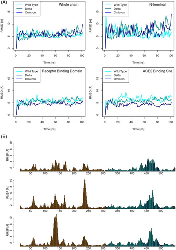
We then compared the three variants Spike molecular dynamics simulation. We use the root mean square deviation (RMSD) observable, calculated over some different portions of the S molecule. The results of this analysis are reported in Figure 3A. The upper left panel regards the whole proteins: after a short equilibration time, all three proteins reach equilibrium with a similar displacement from the initial configuration, highlighting overall comparable stability. In the next three panels (Figure 3B–D) we report the RMSD obtained locally over the NTD, the RBD, and the ACE2 binding site. As evident from the upper right panel, the NTD in all the cases is very mobile: however, it is worth noting that both variants show a behavior more unstable than the wild type. Interestingly, ACE2 appears to present an opposite tendency. Indeed, while the stability of the RBD as a whole is comparable in the three simulations (lower left panel), the mutations seem to lower the RMSD and stabilize the ACE2 binding site (lower right panel), especially for the Omicron case. Moreover, we consider the root mean square fluctuation (RMSF), calculated over each residue of the NTD and RBD in all three molecular simulations. The results can be found in Figure 3B, where the upper, the central, and the bottom panel regard the wild type, the Delta, and the Omicron S protein, respectively. It should be remarked that the variants that improved mobility of the NTD previously discussed have different origins in Delta and Omicron. Indeed, by comparing the three plots it becomes evident that the RMSF of residues around 240 is responsible for the higher mobility of the Delta S protein. Conversely, the omicron RMSF results show very high mobility in the residues around 140, while the peak around 240 disappears. However, the differences in the RBD are less evident: this notwithstanding, looking at the ACE2 binding site residues (blue bars), a decrease in the RMSF of such residues emerges.

It has to be noted that, as known, SARS-CoV-2 Spike protein is mostly covered by glycans and they play an essential role in various aspects of the Spike structure and dynamics. In fact, besides the shielding role shared with other fusion proteins, many authors have hypothesized that they have a functional role in binding with ACE2 or in maintaining a stable conformation of Spike itself.⁶⁵ However, some papers underline that glycans' presence influences the dynamical behavior of the Spike protein on a very long time scale (at least tens of microseconds),^{66, 67} while on shorter time scales, such as the ones we investigated in this work, it seems that their influence is lower.⁶⁸ In addition, we focused on characterizing the binding mechanism between Spike and antibodies: it has been shown that antibody recognition can occur mainly in Spike regions where the glycan shield is not present, thus we considered that the absence of glycans in the Spike simulations was not expected to significantly affect our findings, while allowed for a relevant decrease of the computational cost. In this panorama, we performed two additional 250 ns-long molecular dynamics simulations of the Spike S1 domain, in its WT sequence, one with the glycans and one without them. Overall, the results of these analyses represent a convincing indication that residue mobility on a short time scale is not strongly affected by the presence/absence of glycans (See Data S1).

2.4 Modeling the physico-chemical changes in SARS-CoV-2 variants and their importance for antibody recognition

To further analyze the local differences in the S protein induced by the variants mutations, we introduce two descriptors to quantitatively characterize the local shape and hydrophobicity. For this purpose, we build for each frame of the molecular dynamics simulations the corresponding molecular surface, using the DMS software.⁶⁹ We then exhaustively sample the molecular surface, selecting 10% of its points. Each point is used to determine a patch, defined as the set of molecular surface points closer than a threshold to that point. Finally, we assign each patch to the residue generating its center.

The shape of each patch can be thus characterized in terms of 2D Zernike descriptors, according to a method we recently developed³⁹: the geometrical features of the patch are summarized in an ordered set of numerical descriptors, allowing an easy patch-to-patch comparison applying a standard Euclidean metrics between their descriptors. Moreover, we characterize also the hydrophobicity of a patch: using a residue molecular-dynamics-based hydrophobicity scale we recently published,⁵⁰ the hydrophobicity of a patch is defined as the weighted mean hydrophobicity of the residues generating its points (see “Materials and Methods” for details).

In Figure 4A, we report the results of the shape analysis conducted over the three molecular dynamics simulations of the wild-type and variants of S protein. The top panel concerns the wild-type simulation and highlights which regions on S show the highest shape variability. To measure the shape variability of a patch, we start by calculating its Zernike descriptors for all the frames of the simulation and computing the distances between all these descriptions. The average of such distances quantifies the shape variability this patch experiences along the simulation. Then, we perform a mean on the patches relative to the same residue. Lastly, we standardize our results by subtracting to each residue value the global mean. In this way, we can identify which regions are more variable in shape: a positive high value means a high variability while a negative high value indicates high shape conservation. Looking at the top panel of Figure 4A we confirm the relative instability of the wild-type NTD, overall characterized by a high number of positive peaks. Interestingly, one of the most variable regions in the RBD includes some residues responsible for ACE2 binding.

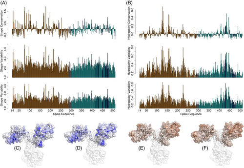
The central and the bottom panels are in Figure 4A represents the shape variability, with respect to the wild type, exhibited by the Delta and Omicron S protein variants, respectively. To obtain these graphs, we characterize each patch of each frame with the Zernike descriptors. As a next step, we calculate the distances between its shape description in all the frames of the considered variant simulation and its shape description in all the frames of the wild-type simulation. In this way, we define a measure of the shape changes between each variant and the wild type. We call this measure the shape variability index. Intuitively, the regions mostly characterized by large shape changes induced by the mutations should be the most unstable in the wild-type case: this is true for both the Delta variant (central panel, Pearson correlation coefficient of 0.90) and the Omicron case (bottom panel, Pearson correlation coefficient of 0.92).

The same analysis is performed in terms of hydrophobicity in Figure 4B: the peculiarity here is that the patch hydrophobicity is summarized in a single numerical value. The top panel regards the wild-type Spike protein simulation, where a high positive value indicates a residue whose patches tend to modify its hydrophobic behavior during the simulation while high hydrophobicity conservation is shown by residues characterized by negative values. Here, even if the lowest conservation is still in the NTD, the exposed regions are equally characterized by low conservation. As in the previous shape analysis, the central and bottom panels of Figure 4B measure the changes exhibited by the variant forms of S with respect to the wild type. Symmetrically, we call this residue-level measure the hydrophobicity variability index of either Delta or Omicron.

To offer a more understandable representation of these results, in Figure 4C, D, we report a molecular representation of the two variants, where the intensity of the blue color is determined by the shape changes with respect to the wild-type. Analogously, in Figure 4E, F the Spike protein of the two variants is colored according to hydrophobicity changes: the higher the intensity of brown the higher the difference experienced in that region by the variant.

2.5 Relationship between physico-chemical changes and immunogenicity

In the previous sections, we characterized the S protein regions both by looking at immunogenicity, (i.e., the frequency with which antibodies bind that region), and variability (i.e., the changes that that region experiences due to the variants mutations). Therefore, each S residue is now described by several indexes: an immunogenicity index reflecting how many times it was experimentally observed in interaction with an antibody; a shape variability index indicating how much the molecular regions surrounding the antibody binding site change their shape because of the mutations in the variants; a hydrophobicity variability index summarizing the chemical changes in hydrophobicity of the patches around the antibody binding site when the variants are considered.

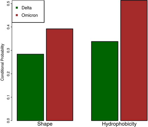
To relate these quantities, we adopt a conditional probability approach. Indeed, if the variant's physico-chemical changes occur in regions characterized by a high antibody binding frequency, it is more likely that the antibodies generated against the wild-type version of S protein cannot recognize anymore the Spike mutated version. Therefore, we want to know the probability of a residue having surface regions highly variable in shape and/or hydrophobicity, conditioned to its high immunogenicity.

We show such probabilities in Figure 5. It emerges that the conditional probabilities obtained by the Omicron variant are higher than the ones of the Delta, both in terms of shape and hydrophobicity. This means the S protein of the Omicron variant is more different from the wild type in the antibody interested regions than the Delta variant: this could imply a more pronounced escape capability from antibodies elicited against the wild-type S protein, as confirmed by literature.^{70, 71}

4.1 Datasets

The Spike dataset was built using CoV-AbDab⁷² and the General dataset with SabDab.⁷³ Separately for both datasets, we selected the antibody complexes with a level of redundancy lower than 90% using cd-hit.⁷⁴ All the structures are renumbered according to Chotia numbering scheme^{10, 11} with an in-house Python script.

The sequences of the original, Delta and Omicron Spike protein have been taken from the GitHub repository of a recent work.⁷⁵ We then modeled the three trimeric structures with Swiss Model,⁷⁶ using the structure deposited in Protein Data Bank⁷⁷ with the code 6vxx as a template.

The Spike NTD comprises residues 1–305. The Spike RBD is composed of residues 319–541. The residues forming the ACE2 binding sites, as defined here,⁴⁴ are 439, 446, 449, 453, 455, 456, 473, 475, 476, 477, 486, 487, 489, 490, 492, 493, 496, 497, 498, 500, 501, 502, 505.

4.2 Nonbonded energy calculation

The partial charges were assigned to atoms using the PDB2PQR software,⁷⁸ with standard options. Before the proper energy calculation, the structures were minimized with Gromacs 2020.6.⁷⁹

4.3 Molecular dynamics simulations

The simulations of the Spike trimers were performed using Gromacs 2019.6,⁷⁹ using the the CHARMM-36 force field.⁸¹ Proteins were placed in a dodecahedric simulative box, with periodic boundary conditions. We used the TIP3P model for water molecules.⁸² In all the systems, all protein atoms were at least at a distance of $1.1\mathrm{nm}$ from the box borders. The minimizations were performed with the steepest descent algorithm. Next, a two-step thermalization of the system was run in NVT and NPT environments each for 0.1 ns at 2 fs time-step. Using the v-rescale thermostat, the temperature was kept constant at 300 K. In the production runs of 100 ns, the pressure was set at $1\mathrm{bar}$ with the Parrinello–Rahman barostat.⁸³ We adopted the LINCS algorithm⁸⁴ to constrain bonds involving hydrogen atoms. Short-range nonbonded interactions were evaluated with a cutoff of $12\mathrm{\AA }$. The Particle Mesh Ewald method⁸⁵ was adopted for the long-range electrostatic interactions.

4.4 Patches definition

All the molecular surfaces used in this work have been calculated using the DMS software with standard parameters.⁶⁹

The center of the patches have been defined using the starting structure of the Spike protein original version, sampling one point per ${\mathrm{\AA }}^2$ from the molecular surface of such structure. Each of the resulting 27 179 points has been used to build a patch. In the starting structure of the wild-type Spike protein, a patch is defined as the set of molecular surface points closer than 6 Å to the patch center. To determine the patch centers in all the other simulation frames and for the variants, we super-positioned each structure with the starting structure of the original Spike. The points closest to the ones selected on this original version were taken as the patches center of that structure. The patch was then constructed using the same threshold of 6 Å.

4.5 Zernike descriptors

Therefore, the set of polynomials forms a basis. The knowledge of all the coefficients $\left\{c_{\mathit{nm}}\right\}$ permits the description of the original function, while the detail level of the description is determined by the order of expansion, $N=\max \left(n\right)$.

The modulus of a coefficient ($z_{\mathit{nm}}=\mid c_{\mathit{nm}}\mid$) does not depend on the phase, being invariant if we perform a rotation around the origin. The $z_{\mathit{nm}}$ is the Zernike invariant descriptors.

The shape similarity between two patches is, therefore, studied by comparing their Zernike invariants. In particular, we measured the similarity between patch $i$ and $j$ as the Euclidean distance between their invariant vectors. We adopted N = 20, therefore dealing with 121 invariant descriptors for each patch.

4.6 Hydropathy of patches

Each point of a patch has been generated from one residue. Each amino acid is characterized by a hydrophobic value.⁵⁰ Therefore each patch point can be associated to the hydrophobic value of the residue generating it. The hydrophobicity of a patch is the mean of all the patch points hydrophobicity.