The morphological variation of acetabular defects in revision total hip arthroplasty—A statistical shape modeling approach
Abstract
Classification and evaluation of acetabular defects remain challenging and are primarily based on qualitative classification methods. That is because quantitative techniques describing variations of acetabular defects and accompanying bone loss volume are not available. This study introduces a new method based on statistical shape models (SSMs) to quantitively describe acetabular defects. This method is then applied to 87 acetabular defects to objectively describe the variations in acetabular defects typically encountered during revision total hip arthroplasty. The absolute bone loss volume, relative bone loss volume, and relative bone loss surface area with respect to the SSM-based pre-diseased anatomy were used to quantify the acetabular bone defects in different segments of the acetabular surface. The absolute bone loss volume of the average defect shape was equal to 37.0 cm3. The first three principal modes, accounting for 62% of the total shape variation, were found to represent variations in acetabular defect morphology. The first, second, and third principal modes described, respectively, the size of the bone defects, the difference between superomedially and superolaterally migrated defects, and the degree of involvement of the posterior or anterior column. The developed SSM and the introduced approach could be used to create automated and unbiased classification methods based on quantitative data. Moreover, the proposed model and the underlying data provide the basis for a quantitative design approach where the shape and size of new acetabular implants are determined according to clinical variation present in acetabular defects.
1 INTRODUCTION
Total hip arthroplasty (THA) is one of the most commonly performed orthopedic procedures. Numbers are projected to increase even further in the upcoming decades1, 2 as joint replacements are being performed in ever younger patients for a still growing range of clinical indications.3 In parallel, improvements in the implant materials, surgical technique, and the peri-operative pathways have further enhanced the success of primary THA.4, 5 However, aseptic loosening remains a major concern, particularly in younger patients.6 Moreover, the incidence of prosthetic joint infection and periprosthetic fracture has not decreased in recent years.7, 8 Hence, the increase in the number of primary THA's is expected to be associated with an increase in the number of revision cases.9
Severe bone loss poses a great challenge in revision THA in terms of establishing primary implant stability, restoring hip biomechanics, and ensuring the long-term survival of the prosthesis while keeping future revision options open. Classification systems are used to define acetabular defects and plan surgical interventions. The most commonly used classification systems are the American Academy of Orthopaedic Surgeons (AAOS), Paprosky, and Gross systems.10 However, no classification method is universally accepted. Moreover, even the most contemporary systems are based on 2D imaging techniques, do not provide quantitative data on the defect, and are often incapable of formulating comprehensive and reliable descriptions of the defects that can be shared between orthopedic surgeons.10 This affects the reporting and interpretation of scientific studies, as well as, their translation to clinical guidelines.11
A better understanding of the acetabular defect morphology could guide the design and sizing of future acetabular implant components. A mismatch between the bone defect shape and implant shape can indeed cause a poor initial fit and stability, which is a requirement for long-term implant survival.12 The search for a good fit in revision total hip arthroplasty has led to the introduction of new solutions such as oblong cups, structural allografts, and porous augments.13-15 However, obtaining acetabular component stability with these solutions is challenging in severe defects as they fail to comply with their large variability in shape.16 If available, an objective description of the variability in acetabular defect shapes could be incorporated in the design or evaluation process of new implant solutions which could lead to better-fitting acetabular components.
In this era of three-dimensional (3D) imaging and advanced processing techniques, it has become possible to take a more quantitative approach to acetabular defects. Several studies have used discrete parameters to describe acetabular defects in revision THA. These parameters include volumetric bone loss, bone formation, and defect ovality.11, 17, 18 These quantitative analyses have paved the way for future and unbiased classification systems and more accurate defect descriptions. However, because of the use of discrete parameters, none of these studies describe the morphology of acetabular defects in its 3D-entirety, that is, by directly describing their 3D shapes, which should be considered the most comprehensive method of all. The latter could be achieved through the use of geometric morphometrics and statistical shape models (SSMs). Recently, we have developed a pelvic SSM and associated method for the reconstruction of acetabular bone defects. Extending such an SSM-based approach to describe the morphology of acetabular defects could give a comprehensive overview of the average acetabular defect shape as well as its variations. This information could provide valuable insights for future classification systems and could guide implant manufacturers during the shaping and sizing of new acetabular components. We, therefore, aimed to (1) extend an SSM-based method to quantitively describe the morphological variations of acetabular defects and (2) apply this method to 87 defects typically encountered in revision THA and present the observed variations.
2 MATERIALS AND METHODS
2.1 Dataset of acetabular defects
To investigate the morphology of acetabular defects, 87 computed tomography (CT) scans of pelvises from patients were retrospectively collected. These patients all underwent two-stage revision surgery due to periprosthetic joint infection at our institution. Acquisition of these scans took place between the excision arthroplasty and subsequent reimplantation stage. This study was approved by the Medical Ethics Committee of the University Hospital Leuven (S61746). Exclusion criteria included scans of patients with a metallic implant in the hemipelvis, pelvic discontinuities, and bony abnormalities unrelated to the acetabular defect, for example, screw fixation of the sacroiliac joint. Furthermore, scans of low resolution that prevented the accurate segmentation of the acetabular defect or where the field-of-view was insufficient to capture the entire acetabular defect were excluded. These exclusion criteria were chosen to reduce the effect of metal artifacts on the segmentation accuracy. Application of the inclusion criteria resulted in the scans of 45 male and 42 female patients being included in the study (age, 66.4 ± 10.0; mean ± SD). The average slice thickness and pixel sizes were 1.3 (±0.5) mm and 0.7 (±0.18) mm, respectively.
2.2 Healthy shape model creation and reconstruction method
The healthy shape model, which is used to reconstruct the pre-diseased anatomy, was previously built from 90 healthy hemipelvises (45 males, 45 females). The healthy shape model construction was unchanged from a previous study in which it was validated.19 In short, the CT scans of these patients were checked for bony abnormalities by an experienced hip surgeon (M. M.). Watertight 3D shapes were constructed after the segmentation of the pelvises from the CT scans models using Mimics Innovation Suite (v22.0, Materialise). Point-to-point correspondence was established using an iterative registration procedure involving both rigid and non-rigid registration steps.20 A Gaussian process morphable model was built using the point-to-point correspondences.21 The Gaussian process model was limited to the first 30 principal component modes and was further augmented with additional variation through a Gaussian kernel. The paired principal component score plots of the first six components can be found in Figure S1. Validation of this shape model was performed using a leave-one-out cross-validation study as described in Meynen et al.19
The reconstruction of the pre-diseased morphology itself was synthesized from the remaining healthy parts of pathologic pelvises. The reconstruction method is based on Markov chain Monte Carlo sampling of both shape and poses parameters to find the best fitting reconstruction candidate.22
2.3 Defect shape model creation
A schematic drawing illustrating the different steps involved in the creation of the defect shape model creation is presented in Figure 1. The pathologic CT scans were manually segmented using Mimics Innovation Suite and were converted to 3D shapes. These shapes were smoothed taking care that anatomical details were preserved upon visual inspection. The pathologic areas were manually annotated on each of the shapes under the supervision of an experienced hip surgeon (M. M.) and were removed from the mesh (Figure 1A). The remaining meshes were roughly aligned with the healthy shape model's mean shape, including a mirroring transformation to account for possible differences in the defect side (left/right). Each of the shapes was reconstructed using the reconstruction workflow to obtain the original (i.e., pre-diseased) pelvis morphology. The reconstructed shape was then registered back to its original position (Figure 1B).

The point-to-point correspondence of the defect shapes was established using a ray-casting procedure in MATLAB (2019b, The Mathworks Inc.). This procedure utilized the existing correspondences of the reconstructed shapes (Figure 1C). To annotate the acetabular surface and acetabular rim in each of the reconstructed shapes, the mean reconstruction shape was defined and both regions were manually annotated. Hereafter, the previously established point-to-point correspondences were used to identify the corresponding acetabular surfaces and rims in each individual reconstructed shape. The hip joint center (HJC) was identified as the center of the sphere fitted to the acetabular surface in each reconstructed shape. Rays were cast from the HJC to each of the points of the acetabular surface to obtain the acetabular depth. For each ray, four scenarios were possible (Figure 2). In the first scenario, the ray is cast through a point of the pre-diseased acetabular rim only and the defect depth is defined as zero. In a second scenario, an intersection is found with the defect shape after first intersecting the pre-diseased acetabular surface. Here, the acetabular depth is defined as the Euclidean distance between both consecutive intersections. The third scenario occurs in the case of bone growth, osteophytes, or reconstruction errors. Here, the ray first intersects the defect surface before intersecting the pre-diseased acetabular surface. The defect depth is then defined as zero. In the fourth and last scenario, no intersection was found with the defect surface indicating that no bone remained. In this case, an interpolation using multi-quadratic radial basis functions was performed to establish the defect surface intersection based on the neighboring remaining defect surface. The defect depth was defined as the Euclidean distance between the interpolated intersection and the acetabular surface. Furthermore, the indices of these points were stored, which in the next step was used to evaluate the risk of complete bone loss. The calculated defect depths were used to construct a defect surface, i.e., a negative of the defect, for each of the defect shapes (Figure 1D).

Each reconstructed acetabular surface was aligned using an unweighted Procrustes analysis, during which the defect surface was deterministically omitted. The mean squared distance was minimized between the corresponding points by a similarity (translation, rotation, and isotropic scaling) transformation. Hereby, all shapes were normalized with respect to the scale of the reconstructed acetabular surface. These transformations were then identically applied to each of the corresponding defect surfaces. For each defect shape, a column vector was constructed containing the reconstruction and defect surfaces, as well as, a Boolean representation of the indices where no defect intersection was found. All column vectors were combined into a data matrix after which the mean column vector was subtracted from each column to center the data. Lastly, principal component analysis (PCA) was applied to the centered data matrix (Figure 1E). To evaluate the assumption of multivariate Gaussian data in the PCA, we visually evaluated the paired principal component score plots of the first six components for non-normality. The shape model performance was evaluated using compactness and generalization measurements.23, 24 The compactness measurement indicates how efficient the shape model can represent variability in the dataset. The generalization measurement quantifies how well the shape model can represent unseen data and can identify if the dataset used to train the model is adequate.
2.4 Analysis of shape variations
The PCA identifies the principal modes of variation (eigenvectors) through the singular-value decomposition of the covariance matrix. In this study, we arbitrarily decided to analyze the three most significant modes of variation that explained approximately 62% of the total variation in the data matrix. The higher modes contributed less than 10% of the defect shape model's total variation and were therefore not evaluated. The statistical significance of the modes was evaluated using a Horn's parallel analysis based on 1000 simulations with a significance level of 0.05.25 The normality of the three first principal component scores was tested using Kolmogorov–Smirnov and Shapiro–Wilk normality tests with a significance level of 0.05. The shape variations were analyzed in both the positive (+2 SD) and negative (−2 SD) directions of all three principal modes representing approximately 95% of the total variation within the data set. The shape variations were assessed in three ways.
First, the 3D shape constituted by the acetabular and defect surface together, that is, the disappeared bone volume, was analyzed qualitatively. Second, we quantitatively evaluated the defect shape using different zones of the acetabular surface. These zones were divided based on a modification of the Wasielewski zones for safe screw insertion (Figure 3).26 The following adaptations were made: (1) a central zone was added, which spanned two-thirds of the acetabular radius (zone 0) to assess the medial acetabular bone loss, and (2) the posterior-superior segment was split (zone I and II) to more precisely assess the variation in the defect direction. For each of these zones, we evaluated the bone volume loss in absolute terms (in cm3) as well as a percentage of the total bone loss variation occurring in the principal mode(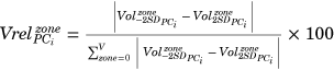 ). Lastly, we analyzed the chance of complete bone loss within each of the zones for the different modes. We used the bone loss data to evaluate the relative amount of surface area, which had a higher than 50% chance of having a complete bone loss. Both the volume and bone loss measurements were fully automated using the existing point-to-point correspondences within Mimics Innovation Suite, preventing possible operator-induced variability.

3 RESULTS
3.1 Shape model performance
The first three modes captured approximately 62% of the total variation in the defect shape model (Figure 4). The parallel analysis identified the first ten modes as statistically significant; they represented approximately 85% of the total variation. The principal component score plots can be found in Figure S2 and revealed no relationships between the components. Visually, all plots are centered around the origin and approximate a Gaussian point cloud. The generalization measurement showed that the defect shape model could explain new unseen defects with an average error of 0.32 mm if all 86 modes were used. The average error increased to 0.95 mm if only the first three modes are used. The first three components did not deviate significantly from the normal distribution.

3.2 Qualitative observed variations
The first principal component (PC1) explained approximately 40% of the total defect shape variation. The main observed variation of PC1 was the size of the defect (Figure 5). The defect size varied for all but the anteroinferior direction. The probability of bone stock remaining at the acetabular rim decreased with increased defect sizes. Similarly, the probability of complete bone loss near the acetabular rim increased for larger defects. The same trend was observed for the central zone (medially) of the acetabulum. The second principal component (PC2) explained approximately 13% of the total shape variation. The observed variation for PC2 was the variation in the superior and medial migration of the acetabular defect. With increased medialization, a higher probability of bone loss at the acetabular fossa was observed. The third principal component (PC3) explained ~10% of the total shape variation. The observed variation for PC3 was the defect direction towards the posterior or anterior column. The 3D STL files of these variations can be found as Supplementary Material.

3.3 Quantitative observed variations
The mean total defect volume was 37.0 cm3 (Figure 6). The three main regions with the largest amount of bone loss were zones 0 (8.6 cm3), I (7.6 cm3), and II (6.8 cm3). As shown in Figure 6A, the first principal component (PC1) varied the total bone loss from 7.3 cm3 (−2 SD) to 85.2 cm3 (+2 SD). A positive variation of PC1 increased the volume of bone loss in each zone, whereas a negative variation decreased the bone loss of each zone. The largest absolute bone loss variation was found in zone I while the smallest bone variation was found in zone IV. The second principal component (PC2) changed the total bone loss from 33.6 cm3 (−2 SD) to 49.4 cm3 (+2 SD). A positive variation of PC2 increased the bone loss in zones I and II, but decreased the bone loss in the other zones (Figure 6B). Inversely, a negative variation of PC2 decreased the bone loss of zones I and II but increased the bone loss of zones 0, III, IV, and V. The bone loss in zone 0 increased from 5.4 cm3 (−2 SD) to 12.3 cm3 (+2 SD). The third principal component (PC3) only varied the total bone loss slightly from 38 to 41.6 cm3 (Figure 6C). A positive variation (+2 SD) in PC3 increased the bone loss most pronounced in zone III. A negative variation primarily increased the bone loss in zone V.

The first principal component (PC1) caused the largest relative variation in zone I, where 28.0% of the total variation was found (Figure 7A). This is in contrast to zone IV, where only 1.0% of the variation occurred. The remaining Zones 0, II, III, and V contributed almost equally to the total variation. The second principal mode variation was largest in zone III and smallest in zone V (Figure 7B). The variation of bone loss of PC3 was largest in zone V and smallest in zone 0 where it only contributed 0.6% of the variation (Figure 7C).

The relative bone loss surface area indicates the percentage of the defect acetabular surface area which has a >50% chance of having no bone remaining. Approximately 15.4% of the average defect acetabular surface has a 50% or higher chance of having no bone remaining. The chance of having no bone remaining was the highest for zone II. As shown in Figure 8A, PC1 increased (+2 SD) and decreased (−2 SD) the surface area with a high chance of no bone remaining to 25.5% and 8.0%, respectively. Zone II continued to have the largest relative surface area with a high chance of no bone remaining in view of these variations. A positive variation (+2 SD) of PC2 decreased the risk of bone loss for zones II, III, and V (Figure 8B). A negative variation (−2 SD) increased the risk of bone loss for all zones, including the central zone 0, where 17.9% of the bone surface had a high chance of no bone remaining. A positive variation of PC3 mainly caused a higher risk of bone loss in zones II and III (Figure 8C). Inversely, a negative variation caused an increased risk in zone V.

4 DISCUSSION
The objectives of this study were to develop a method to describe the variation in acetabular defect morphology using SSMs and apply this method to 87 defects typically encountered in revision THA. Measurements of loss of bone volume and surface areas were used to present the variation in acetabular defects quantitatively.
The dataset used for the defect shape model consisted of CT scans with no metal implant in situ at the time of imaging. The vast majority of the patients had undergone a Girdlestone procedure where no spacer had been left in situ. This choice was made to facilitate the segmentation of the CT scans and improve its accuracy. Segmentation of medical images is hindered in case a metal implant is present, as a result of image artifacts. Furthermore, we primarily wanted to describe the morphology of acetabular defects that needed to be treated after the removal of the primary implant. Nevertheless, the methodology remains applicable in patients with a metallic implant in-situ at the time of CT scan acquisition, such as for example, in case of aseptic loosening of the acetabular component. An evaluation of the bone loss based on scans with the implant in-situ would not identify any bone loss caused during the removal of the previous acetabular component, which could affect the preoperative plan. Furthermore, extra care should be taken during the segmentation of scans with metal artifacts. Needless to say, this methodology can also be applied to patients with acetabular defects of their native hip joints, for example, secondary to septic arthritis, malignancies, or trauma.
In recent years, several studies have quantified the bone loss occurring in patients with osteolytic lesions at the acetabular cup.27-31 Most of those studies report on bone loss in patients with a stable cup, which does not usually require revision surgery. Therefore, the reported bone loss is often lower than the values found in the present study. Garcia-Cimbrele et al.28 evaluated bone loss based on CT scans of 60 patients scheduled for cup revision. The authors reported an average bone loss of 37.9 cm3, which is in agreement with the 37.0 cm3 bone loss found in this study. Schierjott et al. used quantitative analysis to assess the loss of bone volume in 50 acetabular defects. They found a median bone volume loss of 56.8 cm3, which is larger than the bone loss found in the present study. The highest amount of bone loss was measured in the roof of the acetabulum, a zone roughly corresponding to the posterosuperior zone. A median bone loss of 20.5 cm3 was measured, which is more than the average 14.4 cm3 found for the combined zone I and II. The quantitative differences could be attributed to the different methods of measuring bone loss and possible differences in defect severities. The risk of complete bone loss is largest at the superior section of the posterior column. Gelaude et al.32 found the highest relative bone loss in the posterosuperior zone, which is in agreement with the present study. They used similar zones, but they did not further subdivide the posterosuperior zone.
The first three modes of the PCA were used to investigate the variation in acetabular defect morphology. Each mode was varied with two standard deviations, evaluating the variation of ~95% of the variation in the training dataset. The first mode of variation was found to represent the magnitude of the defect, indicated by the variation in bone loss in the posterosuperior direction. This bone loss also affects the entire anterior and posterior columns to a lesser extent. These findings agree with other studies, which have shown that acetabular defects present as multi-directional involving multiple segments of the acetabulum. The second mode of variation represents the variation in the superior and inferior/medial directions. The model thus indicates that defects tend to either migrate more superiorly or medially. This is in agreement with the current understanding of acetabular defects, where the migration of the acetabular component is directed either superolaterally (up-and-out) or superomedially (up-and-in).33 The third principal mode of shape variation represents the involvement of the anterior or posterior column. This mode seems to indicate that the degree of involvement of the acetabular and posterior column is at least partly independent from the other variations in the defect shape.
This study has several limitations. (1) The healthy shape model consisted of pelvises from both males and females. The pelvis has highly sexually dimorphic anatomy, suggesting that a gender-specific model could lead to more accurate reconstructions.34 We were unable to verify this in our study as this would have led to an insufficient number of shapes in each gender-specific model. Further research with a more extensive training dataset is therefore necessary. (2) The dataset for the defect shape model consists of 87 acetabular defects. It is uncertain that this dataset is large enough to capture the large variation in acetabular defects. However, as shown by the generalization measurement, the defect shape model does succeed in representing new shapes with high accuracy. This indicates that the main variations are successfully captured by the training data in the shape model. The three first principal modes of variation are, therefore, not expected to significantly change as more data is included. (3) Acetabular defects from patients undergoing two-stage revisions were used to build the defect shape model. The time between the first surgery and the CT scans was variable and was in some cases more than three months. The potential effect of bone remodeling on the defect shape is uncertain and might be significant. The surgical technique during implant removal and type of implant could have an effect on the amount and variation of acetabular bone loss. These factors have not been investigated in the current study. (4) The method to quantify the bone volume loss did not consider bone growth. In our experience bone growth is often caused by the presence of osteophytes or bone remodeling after bone impaction grafting. Nevertheless, this may result in an overestimation of the bone volume loss in the presented variations.
The study presents a method to evaluate and visualize acetabular defects quantitively and qualitatively and presents the main variations in acetabular defects. The method to evaluate acetabular defects could be a useful tool in preoperative planning, as it allows for a better evaluation of the true bone loss and provides a tool for templating the shape of the native anatomy to be pursued (Figure 9). However, further steps to fully automate this process would be needed for it to be adopted in daily clinical practice. We are currently evaluating if this visualization of acetabular defects translates to better reliability of existing classification systems and hence could facilitate reporting and interpreting clinical guidelines and scientific studies. The presented methodology and use of SSMs in defect classification could thus lead to fully automated and unbiased classifications.

The main variations in acetabular defects identified in this study can additionally guide the design of novel acetabular components and help to optimize the size and shape of existing acetabular augments and implants. Optimized off-the-shelf implants could improve the malfit between the implant and acetabular fit, promoting better implant stability and minimizing the need for extensive reaming of the acetabular defect. The identified variations in defect morphology can give insight into the requirements of new acetabular components in terms of size and shape.
In conclusion, the shape model presented describes the average acetabular defect shape and the variations thereof. This information could guide implant manufacturers during the shaping and sizing of new acetabular cups or augments. The use of a statistical shape model to describe acetabular defects could facilitate the introduction of automated and unbiased classification methods based on quantitative data.
ACKNOWLEDGMENTS
The research for this paper was financially supported by the PROSPEROS project, funded by the Interreg VAFlanders – The Netherlands program, CCI Grant no. 2014TC16RFCB046. A.M. is a SB Ph.D. fellow at FWO (Research Foundation – Flanders) Grant no. 1SB3819N.
AUTHOR CONTRIBUTIONS
Alexander Meynen contributed to the image segmentation, development of the modeling approach, data generation and analysis, manuscript writing, and preparation. Georges Vles contributed to the data analysis, manuscript writing, and preparation. Amir A. Zadpoor supervised the research and contributed to the manuscript writing and preparation. Michiel Mulier supervised the research, contributed to the image segmentation manuscript writing and preparation. Lennart Scheys supervised the research, contributed to the development of the modeling approach, data analysis, manuscript writing, and preparation. All authors have read and approved the final submitted manuscript.