This study proposed that due to their high standing water tables that peatlands would be cold humid islands within their landscape, and especially so relative to farmland on mineral soils. To test this hypothesis, we measured air temperature and humidity at 17 locations along a 7.8 km transect across the UK's largest lowland raised bog from February 2018 to January 2019. Air temperature and humidity were measured hourly for 1 year and supported with spot albedo measurements. The study represented a factorial experiment with respect to sites of measurement, the type of land use (peat vs. arable land) and time of sampling over both the seasonal and diurnal cycles. We show that: (a) That although mean annual temperature was not significantly different between arable and peatlands, the arable land showed a decreased amplitude to its seasonal cycle – this is the reverse of the expected pattern. (b) The albedo of the peatland was significantly lower than that of arable land showing that vegetated peatland still absorbed more solar radiation. (c) The specific humidity was lower on the peatland than on the surrounding arable land. The study showed that while shrubby vegetation exists over a peatland then energy budgets are more likely to be dominated by the lower aerodynamic resistance and lower albedo of the vegetated peatland relative to arable land. Thus, shrub-dominated peatlands will not be a cold humid island in their landscape.

1 INTRODUCTION

Peatlands are known to have the potential to be long-term carbon sinks, but could they also act to modify the way in which incoming solar radiation is distributed at the Earth's surface and so act as cold humid islands within the landscape? Because peat soils can continue to accumulate organic matter, they can continue to sequester atmospheric carbon and so act as long-term sinks of atmospheric carbon (Gorham, 1991). Their ability to continue to grow means that peats are unique among soils and have considerable potential to mitigate climate change. Rydin and Jeglum (2013) estimate that peatlands cover 3% of the Earth's terrestrial surface, but it has been estimated that peatlands could store as much carbon as 500 ± 100 Gt (Gorham, 1991; Loisel et al., 2014; Yu, Loisel, Cahrman, Beilman, & Camil, 2014) as much as the rest of the terrestrial biosphere (IPCC, 2013). Their ability to store carbon has meant that studies of the carbon budget, and perhaps more importantly the greenhouse gas budget, of peatlands have become common (e.g., Billett et al., 2004; Nilsson et al., 2008; Roulet et al., 2007; Worrall, Clay, Burt, & Rose, 2012; Worrall, Reed, Warburton, & Burt, 2003). Research has been able to explore managements that could enhance or restore damaged peatlands to being net carbon sinks (e.g., Clay, Worrall, & Rose, 2010; Herbst et al., 2013). Because of the potential for peatlands to be greenhouse gas sinks, Reed et al. (2013) have viewed peatlands as offering a key ecosystem service, that is, climate mitigation. However, by acting as greenhouse gas sinks, peatlands are only acting upon the climate indirectly, but could peatlands modify the climate directly?

The partitioning of surface energy at the Earth's surface controls the climate that people will experience. The partitioning of net radiation at the Earth's surface can occur in several ways. The possible pathways for energy transfer means that in some environments the net radiation will result in a greater proportion of the incoming energy being partitioned to sensible heat flux (H) compared to the other fluxes and especially compared to the energy transferred to latent heat flux (λE). If an environment partitions in favour of sensible heat flux over latent heat flux this could be expected to lead to greater warming of the air and higher air temperatures in that environment. Alternatively, in some environments more of the net radiation (Rn) will be partitioned into the latent heat flux (λE) leading to comparatively lower specific heat flux (H) and corresponding lower air temperatures. A range of environmental features, including, how wet a soil surface is; how tall the vegetation cover is and the presence of an understorey will control the partitioning of energy in an environment between the soil, sensible and latent heat fluxes.

The balance between the sensible heat (H) and latent heat (λE) fluxes is commonly expressed as the Bowen ratio (Bowen, 1926). Peatlands exist because of their higher standing water table compared to other components of the landscape and so have relatively high water contents at the surface making water relatively more available for evaporation. Therefore, peatlands could be expected to have a lower Bowen ratio (B) than many other ecosystems and would be able to, in comparison to other environments, partition a greater proportion of the incoming energy into latent heat flux. The comparatively low B and lower partition of energy going to H would lead to lower air temperatures other peatlands compared to drier terrestrial environments, that is, peatlands would be cool humid islands.

For bogs in Sweden, Canada and UK, Kellner (2001), Admiral, Lafleur and Roulet (2006) and Worrall, Burt, Clay and Moody (2015) found Bowen ratios (B) were typically below 1, that is, dominated by evaporation (λE). Worrall et al. (2015) considered a UK blanket bog, and estimated the Bowen ratio from long term meteorological observations across 19 years of daily data and found the median monthly Bowen ratio peaked in May–June with values of the Bowen ratio > 1, that is, the dominance of sensible heat flux (H). Conversely, the median monthly Bowen ratio was negative between November and March - a negative Bowen ratio represents times with snow or frozen ground acting as a sensible heat sink (e.g., Kellner, 2001). However, for a six-month period over a New Zealand bog, Campbell and Williamson (1997) measured Bowen ratios of between two and five, that is, sensible heat flux dominated. For comparison, over open water, that is, when latent heat flux should be at its maximum, Rohli, Hsu, Lofgren and Binkley (2004) measured the Bowen ratios between 0.15 and 0.3. Rohli et al. (2004) did observe times when negative values of B were measured over open water, that is, there was domination by evaporative losses and open water could even act as a sensible heat sink. Conversely, for an arid grassland, Ping et al. (2018) found an annual mean Bowen ratio of 1.32. Rejskova, Cizkova, Brom and Jan Pokorny (2012) showed that a wetland exerted a strong cooling effect due to its capacity to convert incident energy to latent heat. Furthermore, Worrall et al. (2015) showed that for a peatland, over 19 years of daily data, λE significantly decreased while H and B significantly increased as the depth to the water table in a peatland increased. Therefore, we propose that a functioning peatland, by virtue of its relatively high water table even with its seasonal variation), will produce cooler air (giving rise to lower air temperatures) more so than other ecosystems such as croplands.

However, change in B is only part of the partitioning of incoming solar energy within an environment. Bonan (2008) has suggested that there are three characteristics of the Earth's terrestrial surface that land cover would influence to control climate. The three characteristics proposed were: the Bowen ratio (B), albedo and surface roughness (as expressed in aerodynamic resistance), although Rigden and Li (2017) have pointed out that these three characteristics could be expected to be correlated and not independent of each other.

Research that has been conducted on the impact of land use on air temperature has dominantly considered the impact of forests in comparison to open land where open land is typically grass or arable land (e.g., Chen & Dirmeyer, 2016). Conversely, there have been few studies of peatlands. In their review of 30 published studies that each considered the impacts of land use or land management, Luyssaert et al. (2014) found only one study that considered the entire energy budget and only four that considered peatlands. Of the four studies only one (Venalainen, Rontu, & Solantie, 1999) considered change in air temperature, however, that study took a modelling approach rather taking any actual field measurements. The results of these studies tend to show that open lands have a higher albedo than forests (Betts & Ball, 1997) but that the open lands have a lower surface roughness (lower aerodynamic resistance) compared to the forests (Rotenberg & Yakir, 2010). Further, forests are thought to have a lower Bowen ratio (B) than open lands and this is due to the comparatively deep roots of trees compared to the shorter vegetation of grass and arable lands. Satellite-based surface temperature studies have shown differences between land use types and managements (Hesselerova, Huryna, Pokorny & Prochazka, 2018; Hesselerova, Pokorny, Brom & Rejskova-Prochazka, 2013). Not included in the review of Luyssaert et al. (2014), Brom and Pokorny (2009) showed that a more vegetated and wetter willow stand on peat soil had a lower air temperature and decreased diurnal temperature compared to a neighbouring meadow in peat. The changes in air temperature due to land use, or land-use change, could be a similar magnitude to those due to greenhouse gas forcing of climate but with the potential to be of the opposite sign (Feddema et al., 2005). Betts, Falloon, Goldewijk and Ramankutty (2007) have modelled the impact of industrialisation on air temperature and shown that deforestation and other land-use change that accompanied industrialisation offset air temperature rise by up to 2 K in northern and mid-latitudes. Subsequent to the review of Luyssaert et al. (2014), Hemes et al. (2018) have shown that that air temperatures over wetlands were lower than on the surrounding drained agricultural, grassland.

Worrall et al. (2019) have shown that upon restoration of a cutover peatland the daytime surface and air temperature declined relative to surrounding arable land. Before restoration the annual average daytime temperatures over the cutover peatland daytime temperatures were 0.7 K warmer than the annual average air temperature over the surrounding arable land – this difference was ascribed to the low albedo of dark peat soils; and a water table in the peatland kept artificially low to aid the digging of the peat. After restoration (including raising of the water table and revegetation with appropriate vegetation), the annual average air temperature over the peatland was either lower or not significantly different from the air temperature over the surrounding farmland and for some parts of the peatland the relative decline in air temperature was 2 K over a 12 year period. Therefore, the hypothesis of this study was that peatlands represent cool islands within a landscape because of their greater capacity to partition net radiation into latent heat flux relative to farmlands. This hypothesis can be tested in a number of ways and we have considered the difference in air temperature, specific humidity and specific enthalpy of the moist air over a peatland compared to its surrounding farmland. More specifically, we would expect that:

Day time air temperatures are cooler over peatlands compared to surrounding arable and that night time air temperatures are warmer over peatlands compared to surrounding arable land. This effect is due to greater partition of incoming energy into latent heat, which means cooler day time air temperatures but the return of some of this latent heat as vapour condenses at night time. This particular prediction does not necessarily mean the daily average temperatures will be lower over peatland compared to surrounding arable land but rather the amplitude of the daily air temperature cycle will be suppressed over the peatland.
Specific humidity will be higher over peatlands than their surrounding arable land as greater availability of water means greater partitioning of incident energy into latent heat and so higher moisture content in the air.
Specific enthalpy of moist air will be higher in peatlands because of the greater partitioning into latent heat.

2 MATERIALS AND METHODS

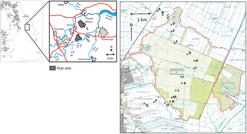
The study considered a transect of air temperature and relative humidity across Thorne Moors,¹ which is the largest lowland peat complex in England (Figure 1) from the farmland on mineral soils on one side of the peatland to the farmland on mineral soils on the opposite side. Thorne Moors, as well as being the largest lowland bog in England it is also in an area of flat land where differences in air temperature due to altitudinal differences will be minimal – the maximum altitude across the study transect was 4 m above ordinance datum (aOD) at site A (Figure 1) and a minimum of 1 m aOD at site I.

Details are in the caption following the image — **FIGURE 1**
Open in figure viewer PowerPoint

Location of Thorne Moors and the transect of stations used in the study. Letters refer to the location of study sites

2.1 Study site

The peatland on Thorne Moors is a 23 km² of former raised bog. Commercial digging of the peat for horticultural uses started on Thorne Moors in the 1870s and finished in 2004 when the Moors, in its exploited state, came under the control of the UK government's nature conservation agency for England (Natural England). The base of the peat on the site has been dated from wooden artefacts to be 3,580 ± 108 Calendar years BP (Shotton and Williams, 1973). Given that Parsons (1878) recorded pre-exploitation peat depths on Thorne Moors of up to 6.1 m then the long-term accumulation rate would be approximately 1.7 mm/year. However, the presence of a Neolithic trackway on neighbouring Hatfield Moors (a few km south of Thorne Moors) has been dated from 4,500 to 4,900 years BP (Chapman & Gearey, 2013) and that would imply a slower average accumulation rate. When Thorne Moors came under government control in 2004, the peat depth was thought to be 0.5 m across the site although (Clay & Worrall, 2015) sampled and characterised two peat cores from Thorne Moors in 2013.

Once coming into government ownership restoration began and water tables were raised by ditch-blocking and revegetation with suitable peatland vegetation was allowed. In 2013, a second phase of restoration started with particularly focused upon scrub removal. Monitoring of water table depth and vegetation cover across the peatland is discussed below.

The surrounding arable land is drained by pumping maintained by the Shires group of internal drainage boards (www.shiregroup-idbs.gov.uk). The surrounding arable land is on the Blacktoft soil series, a calcaric fluvic endogleyic cambisol (Cranfield University, 2020).

2.2 Meteorological measurements

Air temperatures and relative humidity were monitored across along a transect using tiny tag 2 plus loggers (Gemini data loggers, Chichester, West Sussex, UK). The loggers have a reading resolution of 0.1 K and 0.3% relative humidity and a manufacturer's stated accuracy of 0.3 K and 3% relative humidity at 293 K. The loggers were programmed to record relative humidity and air temperature every hour from February 1, 2018 to January 31, 2019. The loggers were positioned to be 1.7 m aboveground, shielded and vented; and all positioned facing north. Before deployment, all loggers were operated at the same location for 2 weeks so that they could be calibrated against each other. Equally, at the end of the experiment remaining loggers were again brought to a common location and left to run together to test for drift and calibration. Neither phase of calibration showed significant differences between loggers or between the beginning and end of the experiment. In total 21 loggers were used at 17 sites across the study transect, which meant that at the outset of the experiment four sites in the study were measured in duplicate.

The relative humidity and air temperature data were converted to specific humidity (θ) and the enthalpy of the moist air (H_s):

θ = \frac{ω}{(1 + ω)},

(1)

ω = \frac{0.622 e_{a}}{(P - e_{a})}

(2)

RH = \frac{e_{a}}{e_{sT}},

(3)

e_{sT} = 0.611 \exp [\frac{(17.67 T)}{(243.5 + T)}],

(4)

H_{s} = (1.006 T - 0.026) + θ (1.84 T + 2501),

(5)

where: T = air temperature (°C); RH = relative humidity; θ = the specific humidity (kg water/kg dry air); ω = the mixing ratio; e_a = actual vapour pressure (Pa); e_sT = saturated vapour pressure at temperature T (Pa); P = atmospheric pressure (Pa); and H_s = specific enthalpy of moist air (kJ/kg). The monitoring sites across the transect were no more than 6 m above sea level and so atmospheric pressure was assumed to be 101.3 Pa.

2.3 Albedo

As a means of understanding the change in the partitioning of incoming energy across the study landscape, albedo was measured at each site (17 sites) on each visit from July 2018 to the end of the experiment, except for the visit in the month of October. On each visit albedo was measured using an pyranometer (MP100, Apogee Instruments, Logan, UT) and was measured as the blue sky albedo, that is, the ratio of the incident radiation to the reflective radiation with the incoming radiation measured as perpendicular to the Earth surface. On each visit to each of the 17 transect sites the albedo was measured five times. The five albedo measurements for each site and each visit were analysed by analysis of variance (ANOVA) as described below.

Although the pyranometer used had no error for solar zenith angles up to 75°, the albedo as measured in this study could be expected to vary with the time of day and year, that is, as solar zenith angle varies. Therefore, all albedo readings were adjusted to local noon by use of the clear sky calculator app (Apogee Instruments, Logan, Utah, USA) and by use of a reference site. The reference site was lawn grass and the albedo of this surface was measured in exactly the same manner as for the field site but deliberately measured across a range of hours from 7 a.m. to 5 p.m. GMT. Analysis of variance of this reference dataset showed no significant difference in relative albedo between 9 a.m. and 5 p.m. GMT.

In addition, to albedo measurements of the study locations, measurements of the albedo of a bare peat area were made upon each visit to Thorne Moors. On one occasion in January 2019 it was possible to measure the albedo of fresh snow. The measurements of the albedo of bare peat and snow were not included in the analysis of the experimental design, rather being included here for comparison.

2.4 Experimental design

The study established 17 sites for monitoring of air temperature and relative humidity. The 17 sites lay on transect that stretched from 1 km north west of the peatland to 1 km south west of the peatland. The transect was designed to be symmetric about a point that was a priori taken as the centre of the peatland (Point I – Figure 1). The transect had eight sites north of the centre point and eight points south of the centre point, on each arm of the transect there were five sites on peat and the final three sites were on arable land. The sites on arable land were positioned to be along field margins, both to avoid damage and interference with agriculture, but also so that depth to water table could be observed from the water level in the drain at the field margin. However, this latter fact would mean that depth to water table at the monitoring would be lower than experienced on the rest of the arable land.

The study was designed as factorial design with five fixed factors. The first factor is the difference between the monitoring sites, henceforward referred to as Site. The Site factor had 17 levels, one for each location on the transact. The second factor is the difference between the land types covered by the study (henceforward referred to as Type) and the land types for this study were classified to give this factor two levels: peatland and arable land. Note that land type factor is both soil type (peat and mineral soils) but also a difference in land use and it is not possible to separate these. The third factor was the difference between month of sampling, henceforward referred to as Month, and this had 12 levels one for each of the calendar months. The fourth factor was the hour of the day, henceforward referred to as Hour, which had 24 levels, one for each of the day. The fifth factor was difference between transects. Although it was one continuous transect, the transect was designed to be duplicated about the centre at position I with eight sites in two transects, that is, this factor had two levels henceforward referred to as north and south. The nature of the factors means that some are nested within each other and it would not be appropriate to analyse them together and so for each property measured a number of ANOVA were applied.

Prior to ANOVA was performed, outliers were identified using a Q-Q′ plot and the Anderson-Darling test used to test for normality (Anderson & Darling, 1952), if data were shown not be normal they were log-transformed and re-tested – further transformation did not prove necessary. The application of the Levene test to the datasets showed that the assumption of homogeneous variance in ANOVA was reasonable. The generalised ω² approach of Olejnik and Algina (2003) was used to calculate magnitude of effects. Values from the ANOVA are presented as least-square means (otherwise known as marginal means). To evaluate differences between the levels of factors and interactions that were found to be significant were post hoc tested using the Tukey test. Unless otherwise stated significance refers to being significantly different from zero at the 95% probability (p < .05).

2.5 Additional data

The hypothesis of this paper is that peatlands represent cool humid islands in a landscape because of high water tables relative to other ecosystems. The available water table and vegetation cover data have been analysed and discussed in Worrall et al. (2019) but are related here for comparison. Water table monitoring was initiated at 48 locations across Thorne Moors in 2013 and the depth to the water table was measured every month from 2013 until 2017. Analysis of variance was used to assess the impact of two factors on the depth to the water table: first, the difference between years (henceforward referred to as the Year factor) with four levels one for each year between 2014 and 2017 inclusive; and second, the difference between months of water table measurement with 12 levels and henceforth referred to as the Month factor. The ANOVA was performed as described above.

Restoration of Thorne Moors was based upon the restoration by revegetation of bare soil and later the removal of scrub; therefore, monitoring of restoration focused upon these aspects of the habitats and characteristics of the Moors. Monitoring of bare soil, open water and scrub cover took place in 2002, 2013 and 2016. In 2002 and 2016 more detailed vegetation surveys were conducted by ground-truthing aerial images. These more detailed surveys meant that it was possible to assess the area of woodland, bare peat, open water, scrub (here defined as areas of vegetation between 0.5 and 3 m in height), grasses, sedges, heather, bracken and the area of non-peat soils.

There are no vegetation surveys on the arable areas included in this study. In the year of study the fields surrounding the transect sites on both the north and south transects were planted with winter wheat (Triticum aestivum). During the study harvest occurred between the July and August visits to the arable sites on both the north and south transect arable sites, and ploughing occurred before the November visits.

3 RESULTS

3.1 Habitat change

The 2017 survey showed that the measured habitats were: woodland (11%), bare peat (9%), open water (11%), scrub (11%), grasses (4%), sedges (10%), heather (Calluna vulgaris - 14%), bracken (25%), non-peat soils (2%) and non-soil areas (eg. trackways - 3%). All peatland transect sites were situated on peat areas without bare soil in the visible vicinity and away from open water and scrub thus they were dominated by – grasses, sedge, heather and bracken. The area of bare peat has decreased overall from 14.8 km² in 2002 to 3.1 km² in 2017. The area of open water rose from 2002 to 2017 – an overall increase of 2.3 km². The increase in the area of open water could be due to the raising of water tables after restoration. However, given the shallow nature of the open water on the Moors (typically 50 cm deep at maximum), the area of open water could alter radically depending upon the time of year or the antecedent weather conditions prior to any survey. The survey was over the summer in 2002, while in 2013 and 2016 the surveys were in early spring (February and March), that is, the initial survey was at a time when one might expect low water tables and so a lower area of open water in the shallow cells/pools that exist on the Moors compared to what be naturally expected in early spring. The area of scrub has increased over the course of the study period – an overall increase of 2.2 km² with an increase of 0.1 km² since 2013. These habitat surveys show that since restoration bare soil has declined from 44% of the area of the Moors to just 9% - a 79% decline; equally, open water has risen from covering 4.4% of the Moors to 11.1% of the Moors in 2017. The changes seen over the period of the study are consistent with the restoration of peatland with higher water tables and more complete vegetation cover.

3.2 Depth to the water table

Both factors (Year and Month) included in the ANOVA were found to be significant (p < .05, R² 10.17%). Eight locations out of 48 had least-square mean water tables above the surface. The second most important factor was Month with water tables in February and March closest to the surface, after which water tables declined with each subsequent month to a low in October of −0.206 ± 0.020 m. The third most important factor was the Year. Given the fact that the data only covered 4 years, it would not be possible to assess any trend in the depth to the water table. Although no direct measurements of depth to water table were made in the arable lands at no stage were water levels in ditches observed to be nearer the surface than 2 m.

3.3 Albedo

In total, there were 701 measurements of albedo (Table 1). Petzold and Renez (1975) give albedo values for a range of surfaces in a Canadian sub-Arctic peatland environment and values reported range from 0.07 (standard deviation = 0.006) for bare surface to 0.26 (standard deviation = 0.2) for a dry lichen surface – there was no Calluna vulgaris or Eriophorum spp. in this study. Miranda (1982) did measure albedo for Calluna vulgaris and measured the average albedo for the dry canopy of 0.11 (95% C.L. 0.09 to 0.13), and for wet canopy, it was 0.18 (95% C.L. =0.15 to 0.21). Piggin and Schwerdtfeger (1973) measured albedo for wheat and barley across a year and found daily albedo values ranged from 0.13 to 0.25 for wheat and from 0.14 to 0.36 for barley. Note that for data from these literature studies we have to accept the form of uncertainty and variation each has used.

TABLE 1. Summary of the albedo measurements across the study period

Surface type	N	Median	95th percentile range
Arable	196	0.22	0.11–0.54
Peat	438	0.19	0.08–0.38
Bare peat	56	0.08	0.05–0.14
Snow	10	0.68	0.51–0.83

For this experiment, when Type and Month were considered then both factors and their two-way interaction were found to be significant (p < .05), with the most important factor being the Month (23% of the original variance, followed by the two-way interaction (Type*Month – 8% of original variance) and least important, but still significant, was the Type factor (4% of the original variance). The interaction term shows that of the 6 months of data for September, December and February the arable land had significantly higher albedo than the peatland, in August the albedo of the peatland was higher than that of the arable land, while for July and October there was no difference (Figure 2). By the timing of the August, measurements harvest had occurred on the arable land but stubble and brash were left on the ground, by November the soil was ploughed and albedo had decreased on arable land sites.

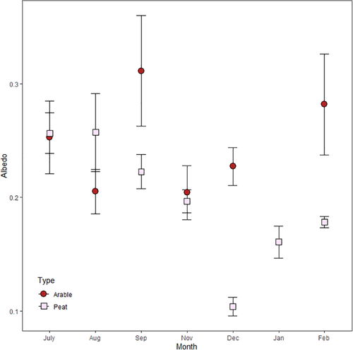
When the Site and Month factors were considered then both factors and their two-way interaction were found to be significant with the most important being the interaction term (Site*Month – 31% of original variance), followed by Month (23% of the original variance) and then the site factor (10% of the original variance). The post hoc comparison shows that study sites exist in four groups (Table 2). The four groups do overlap in their membership, the high albedo group is not exclusively arable land sites but all the arable land sites are in this group. Similarly, the lowest albedo group is exclusively made up of peat sites, and the lowest group is made up of the central site and the sites from the northern transect. A significant lower albedo across the study period does mean that the peatland sites, on average, absorbed more of the incident energy.

TABLE 2. The post hoc comparison by Tukey test for the albedo of the study sites

Site	Type	N	Mean	Group
Q	Arable	34	0.25	1
M	Peat	44	0.25	1
C	Arable	25	0.25	1	2
B	Arable	33	0.24	1	2
A	Arable	39	0.23	1	2	3
P	Arable	35	0.23	1	2	3
O	Arable	30	0.22	1	2	3
D	Peat	25	0.22	1	2	3
K	Peat	45	0.21	1	2	3
J	Peat	44	0.21	1	2	3
L	Peat	43	0.21	1	2	3
N	Peat	45	0.20	1	2	3
E	Peat	35	0.19	1	2	3	4
F	Peat	35	0.18		2	3	4
I	Peat	39	0.18			3	4
H	Peat	44	0.18			3	4
G	Peat	39	0.13				4

Note: The site code letter refers to Figure 1. If sites share a group number they are not significantly different from each other.

3.4 Air temperature

There were 109,769 measurements of air temperature over the study period. Insufficient data came from site B (Figure 1) for it to be included. The air temperature data were normally distributed. The three-way ANOVA considering Type, Month and Hour factors showed that only two factors and one two-way interactions were significant. The most important factor was Month, followed by Hour with Type not being significant. The fact that the Type factor was not significant demonstrates that there was no difference in the air temperatures for peat- and arable-land, but it should be re-stated that the hypothesis stated by this study does not require, nor even expect, the average temperature on peatlands to be lower than that on arable land.

The interaction term Hour*Type was significant and critically it showed that the diurnal cycle in air temperature was different between the peatland and arable land, but that the amplitude of diurnal cycle was significantly smaller in magnitude for the arable land when compared to peatland (Figure 3a). The nature of this significant interaction shows that, when judged across the entire study, period peatlands had cooler air temperatures at night than the arable land, and equally, arable lands had significantly lower daytime temperatures across the study period during daylight than peatlands – this is the reverse of the hypothesized effect and the reverse of the effect observed by Brom and Pokorny (2009) for a comparison between willow and meadow vegetation both on peat soils.

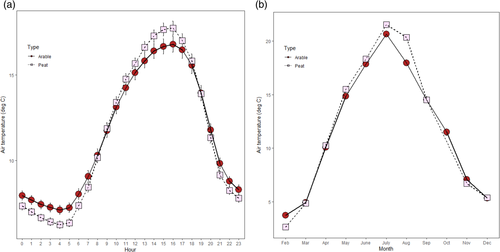
When the Type*Month interaction was considered then the only significant difference between arable- and peat-land was in August with arable land again cooler than peatland (Figure 3b), this would have been harvest time when albedo of the arable would have dominated by ripe wheat and the stubble from harvesting.

Both the arable and the peatland had the same timing for the diurnal air temperature, that is, minimum at 4 a.m. and maximum at 4 p.m. (henceforward to avoid confusion referred to as 0400 and 1600 hr). Therefore, to further test the controls on the air temperature the data were subset to be only for those specific times and reanalysed using only the Type and Month factors. For air temperature at 0400 hr there was a significant Type factor and the least square means confirmed that arable land was on average 0.9 K warmer than the peatland at night time (Figure 4a). The interaction term Type*Month at 0400 hr shows a more mixed picture with arable land being warmer than peatland in February, and September through December, but peatland was warmer than arable in August and there being no difference in all other months. Note that the Type*Month interaction does not follow day length for Thorne Moors – on 21st June 2018 sunrise was 0337 hr GMT.

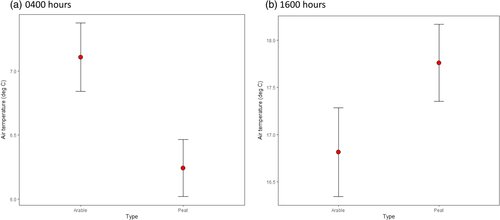
For 1600 hr, the ANOVA shows that peatland was on average 0.9 K warmer than the arable land (Figure 4b). For the interaction term Type*Month, the ANOVA showed that the significant differences were only in the months June, July and August, and there was no month where arable land was warmer than the peatland for this time of the day.

When the Site factor was considered instead of the Type factor for the entire dataset, the Site was significant but it was only the fourth most important term in this general linear model behind Month, Hour and the interaction term Month*Site. The Site term shows there are differences between most sites (Figure 5) but post hoc testing shows that there is high air temperature group of which all three of the arable land sites from the southern transect are members of this group (O, P and Q – Figure 1). Conversely, the three arable land sites on the north transect (A, B and C – Figure 1) were in the six coolest sites, including the coldest site of all the study sites. The post hoc comparison, therefore, implies that part of the effect being observed might be asymmetric with warm air coming from the south west (perhaps having warmed across the urban centres of Doncaster and Thorne) and cooling across the peatland. The Site*Month term shows that for many months there was no significant difference between sites (March through June, and October to November).

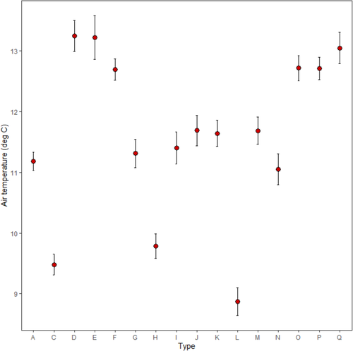
Including transect as factor, there was a significant difference (p < .05) between transects at 0400 hr with the north transect (6.2°C) to the south transect (7.0°C), but there was no significant difference (p > .05) between transects at 1600 hr.

3.5 Specific humidity

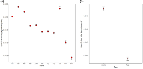
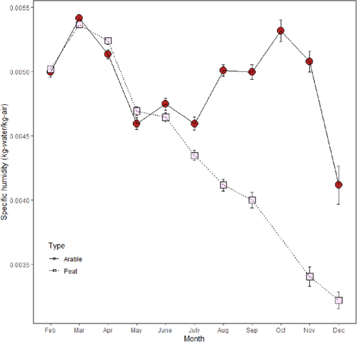
The distribution of θ was not normal and the data were log-transformed prior to analysis. The three-way ANOVA of Type, Month and Hour showed all three factors to have a significant effect and similarly for both interaction terms. The most important term was the Month factor (11% of original variance explained) followed by Hour (9%); Month*Type (8%); Type (6%) and finally the Type*Hour interaction (1%). The main effects plots show that θ peaked in March and declined to a minimum in December (Figure 6a). The values of θ were lower over peatland compared to arable land with the effect being 0.0004 kg of water/kg of air – this again is the opposite of that we have hypothesized (Figure 6b). The interaction term Type*Hour was weak and showed no visible change in the diurnal pattern between peatland and arable land. The Type*Month interaction does show the considerable difference between the arable and peatland, with the largest differences between peatland and arable land being in the summer through autumn (Figure 7).

3.6 Specific enthalpy

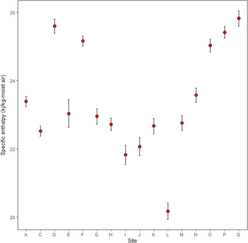
Given the derivation of H_s [Equation (5)] it is perhaps not surprising that the pattern in H_s follows that in θ. The distribution of H_s was not normal and the data were log-transformed prior to analysis. The three-way ANOVA of Type, Month and Hour showed all three factors to have a significant effect and similarly for both interaction terms. The average H_s is 24.14 ± 0.08 kJ/kg of moist air for arable land and 23.14 ± 0.08 kJ/kg of moist air peatland although Type was the least important of the factors, as judged by the percentage of variance explained by that factor. The most important factor was Hour, followed by Month and then the Month*Type interaction. The H_s peaked in July, was at a minimum in December; and peaked at 1700 hr and was at a minimum at 0500 hr. When Site was considered instead of Type as a factor then there was a significant difference (p < .05) between many but not all locations across the transect (Figure 8). There is a plausible asymmetry in the pattern of H_s across the study sites with highest value of H_s at site Q declining to site I.

4 DISCUSSION

We have proposed that on the basis of a relative high water table compared to the surrounding landscape that B (Bowen ratio) is relatively low. A relatively low B leads to a relative reduction in H, the sensible heat flux, and this means a lower air temperature. This study has shown the reverse of that hypothesized, with the diurnal cycle in air temperature having a smaller amplitude on the arable land that surrounds the study peatland than on the study peatland itself. The peatland was warmer during the day and cooler at night than the surrounding arable land. The hypothesis of this study was based solely on differences in B, the Bowen ratio, and given Bonan (2008) has proposed that land cover influences surface climate through three characteristics (albedo, surface roughness and the Bowen ratio) then the other two factors should be considered. The albedo, the surface roughness (as described as aerodynamic resistance) and the Bowen ratio control the air temperature in the following ways:

R_{n} = (1 - α) S_{in} + L_{in} - εσ T_{s}^{4},

(6)

H = ρ c_{p} \frac{(T_{aero} - T_{air})}{r_{aero}},

(7)

λE = \frac{H}{B},

(8)

where: α = albedo; S_in = incident shortwave radiation (Wm⁻²); L_in = incident longwave radiation (Wm⁻²); e; s = Stefan-Boltzmann constant (5.67 × 10^–8 W m⁻² K⁻¹); T_s = surface temperature (K); T_air = air temperature (K); T_aero = aerodynamic temperature (K); r_aero = aerodynamic resistance (s m⁻¹); ρ = density of air (kg m⁻³); c_p = heat capacity of air (J kg⁻¹ K⁻¹).

With respect to albedo this study can show that there was a difference between peatland and arable land with arable land having a higher albedo and in comparison to each other the peatland would have absorbed 3% (1–5% 95th percentile) more energy than the arable land.

Lhomme, Katerji, Pérrier, and Bertolini (1988) showed that in neutral conditions it can be assumed that the roughness lengths for momentum and sensible heat are the same, the aerodynamic resistance above the canopy can be related to canopy height (Allen, Pereira, Raes, & Smith, 1998):

r_{aero} = \frac{\log_{e} [\frac{z_{m} - d}{z_{om}}] \log_{e} [\frac{z_{h} - d}{z_{oh}}]}{k^{2} u_{z}},

(9)

where: r_aero = aerodynamic resistance (s m⁻¹); z_m = height of wind measurements (m); z_h = height of humidity measurements (m); d = zero plane displacement height (m); z_om = roughness length governing momentum transfer (m), z_oh = roughness length governing transfer of heat and vapour (m); k = von Karman's constant, (=0.41), u_z = wind speed at height z (m s⁻¹). Where:

d = \frac{2 h}{3},

(10)

z_{om} = 0.123 h,

(11)

z_{oh} = 0.1 z_{om},

(12)

where: h = canopy height (m).

Peat vegetation on Thorne Moors was surveyed in 2017 and detailed above (woodland [11%], bare peat [9%], open water [11%], scrub [11%], grasses [4%], sedge [10%], heather [14%], bracken [25%], non-peat soils [2%] and non-soil areas [eg. trackways - 3%]). Since the study only monitored on vegetated peat then the peatland sites were mainly in amongheather (Calluna vulgaris) and sedges (dominantly Eriophorum spp.). When compared to wheat both heather and sedges are persistent vegetation so although leaves dieback slightly in winter the canopy height (h) remains close to constant and given the maturity of the vegetation we assume a value of 37.5 cm (Gimingham, 1989). Conversely, the winter cropping in the surrounding arable land the canopy height would be zero in autumn and rise to 50 cm in summer. Assuming that the canopy heights follows a simple linear growth pattern (Figure 9a) then given Equations 9-12) then the annual average r_aero over arable land (average = 44.2 s m⁻¹) would be 112% higher than that on the peatland (average = 20.8 s m⁻¹) (Figure 9b). Therefore, sensible heat flux (H) would be higher over the peatland than the arable land given the nature of vegetation cover across this study transect.

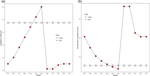
Worrall et al. (2019) showed that restoration of the same dug over peatland as in this study caused a decline in the air temperature over the peatland relative to the surrounding arable land but this study observed no difference. However, the study of Worrall et al. (2019) was comparing air temperatures recorded between 1000 and 1100 hr each day, as dictated by the nature of remotely sensed land surface temperature data used in that particular study, when this study would suggest no difference. Furthermore, the study of Worrall et al. (2019) was comparing a dug over peatland in the year 2000 with vegetated peatland in 2018. The time courses of the relative change in temperature was that the dug over peatland had an annual average 0.7 K warmer than the surrounding farmland; after 2005 the annual average temperature was never greater on the peatland again and in 2016 the peatland was 0.5 K cooler than the surroundings. However, for all years since 2005 apart from 2016 there was no significant difference between the annual average temperatures on the peatland compared to the surrounding farmland. This study would suggest that the transition from dug over peat (bare peat – albedo = 0.08 – Table 1) to the current surface (albedo = 0.19 – Table 1) would have meant a 12% decrease in the energy absorbed by the peatland that it would have had to redistribute through other energy transfers. The dug over peat would have been a dry surface with water table kept low to enable working and albedo of soils is known to decrease with increasing soil moisture (Idso, Jackson, Reginato, Kimball, & Nakayama, 1975). The water table will have risen, although the change in water table depth over the period since 2000 is not known, this will have decreased the sensible heat flux (H). However, the surface roughness will have increased as vegetation developed. This present study would suggest that, when compared to the arable land, the lower albedo and the different surface roughness are dominating the comparative energy balance over the impact of the higher water table. The importance of the shrubby vegetation over the impact of water table change would suggest that for sandy heath environments, where there is shrubby vegetation cover (often Calluna vulgaris) but well-drained soils, then there would be considerable heating effect and sensible heat fluxes would be comparatively even higher. Conversely, in a peatland environment without the shrubby vegetation cover, for example, sphagnum mosses, then the impact of a higher water table controlling latent heat flux and the Bowen ratio may dominate over sensible heat fluxes due to taller vegetation.

5 CONCLUSIONS

This study proposed that peatland, by virtue of its high standing water table, would have lower day time and warmer night time temperatures than its surrounding agricultural landscape. However, this study showed that:

Although there was no overall significant difference in the daily average air temperature experienced across the arable and peatlands the amplitude of the diurnal cycle across for the arable land was lower than that on the peatland. The arable land was on average 0.9 K warmer at night and 0.9 K cooler during the day – the reverse of that hypothesized.
The albedo was lower on the peatland compared to arable land and so peatland would have absorbed 4% more incident energy than the surrounding agricultural land.

Perennial shrubby vegetation on the peatland means the aerodynamic resistance was 63% lower on the peatland, which will enhance the vertical transfer of air over the peatland meaning greater transfer of sensible energy, which would explain higher air temperatures and lower specific humidities.

ACKNOWLEDGEMENTS

The authors are grateful to Hinchliffe and Birtwistle Farms for access to their land throughout the study.

Endnote

¹ By local convention Thorne Moors is always referred to in the plural.

Open Research

DATA AVAILABILITY STATEMENT

Data available on request from the authors: the data that support the findings of this study are available from the corresponding author upon reasonable request.

REFERENCES

Admiral, S. W., Lafleur, P. M., & Roulet, N. T. (2006). Controls on latent heat flux and energy partitioning at a peat bog in eastern Canada. Agricultural and Forest Meteorology, 140(1–4), 308–321.
10.1016/j.agrformet.2006.03.017
Web of Science® Google Scholar
Allen, R.G., Pereira, L.S., Raes, D., & Smith, M. (1998). Crop evapotranspiration-guidelines for computing crop water requirements. FAO Irrigation and Drainage Paper No. 56, Rome.
Google Scholar
Anderson, T. W., & Darling, D. A. (1952). Asymptotic theory of certain “goodness-of-fit” criteria based on stochastic processes. Annals of Mathematical Statistics, 23, 193–212.
10.1214/aoms/1177729437
Web of Science® Google Scholar
Betts, A. K., & Ball, J. H. (1997). Albedo over the boreal forest. Journal of Geophysical Research – Atmospheres, 102(D24), 28901–28909.
10.1029/96JD03876
Web of Science® Google Scholar
Betts, R. A., Falloon, P. D., Goldewijk, K. K., & Ramankutty, N. (2007). Biogeophysical effects of land use on climate: Model simulations of radiative forcing and large-scale temperature change. Agricultural and Forest Meteorology, 142(2-4), 216–233.
10.1016/j.agrformet.2006.08.021
Web of Science® Google Scholar
Billett, M. F., Palmer, S. M., Hope, D., Deacon, C., Storeton-West, R., Hargreaves, K. J., … Fowler, D. (2004). Linking land-atmosphere-stream carbon fluxes in a lowland peatland system. Global Biogeochemical Cycles, 18(1), GB1024.
10.1029/2003GB002058
Web of Science® Google Scholar
Bonan, G. B. (2008). Forests and climate change: Forcings, feedbacks, and the climate benefits of forests. Science, 320, 1444–1144.
10.1126/science.1155121
CAS PubMed Web of Science® Google Scholar
Bowen, I. S. (1926). The ratio of heat losses by conduction and by evaporation from any water surface. Physical Review, 27(6), 779–787.
10.1103/PhysRev.27.779
CAS Google Scholar
Brom, J., & Pokorny, J. S. (2009). Temperature and humidity characteristics of two willow stands, a peat meadow and a drained pasture and their impact on landscape functioning. Boreal Environment Research, 14, 389–403.
Web of Science® Google Scholar
Campbell, D. I., & Williamson, J. L. (1997). Evaporation from a raised peat bog. Journal of Hydrology, 193(1-4), 142–160.
10.1016/S0022-1694(96)03149-6
Web of Science® Google Scholar
Chapman, H. P., & Gearey, B. R. (2013). Modelling archaeology and Palaeoenvironments in wetlands. Oxford, England: Oxbow Books.
Google Scholar
Chen, L., & Dirmeyer, P. A. (2016). Adapting observationally based metrics of biogeophysical feedbacks from land cover/land use change to climate modelling. Environmental Research Letters, 11(3), 034002.
10.1088/1748-9326/11/3/034002
Web of Science® Google Scholar
Clay, G. D., & Worrall, F. (2015). Estimating the oxidative ratio of UKpeats and agricultural soils. Soil Use & Management, 31(1), 77–88.
10.1111/sum.12155
Web of Science® Google Scholar
Clay, G. D., Worrall, F., & Rose, R. (2010). Carbon budgets of an upland blanket bog managed by prescribed fire – Evidence for enhanced carbon storage under managed burning. Journal of Geophysical Research – Biogeosciences, 115, G04037.
10.1029/2010JG001331
CAS Web of Science® Google Scholar
Cranfield University 2020. The Soils Guide. Cranfield University, UK. Retrieved on 03/09/2020 from www.landis.org.uk.
Google Scholar
Feddema, J. J., Oleson, K. W., Bonan, G. B., Mearns, L. O., Buja, L. E., Meehl, G. A., & Washington, W. M. (2005). The importance of land-cover change in simulating future climates. Science, 310(5754), 1674–1678.
10.1126/science.1118160
CAS PubMed Web of Science® Google Scholar
Gimingham, C. H. (1989). Heath and heathlands. Botanical Journal of the Linnean Society, 101(3), 263–268.
10.1111/j.1095-8339.1989.tb00160.x
Web of Science® Google Scholar
Gorham, E. (1991). Northern peatlands: Role in the carbon cycle and probable responses to climate warming. Ecological Applications, 1, 182–195.
10.2307/1941811
PubMed Web of Science® Google Scholar
Hemes, K. S., Eichelmann, E., Chamberlain, S. D., Knox, S. H., Oikawa, P. Y., Sturtevant, C., … Baldocchi, D. D. (2018). A unique combination of aerodynamic and surface properties contribute to surface cooling in restored wetlands of the Sacramento-san Joaquin Delta. California. Journal of Geophysical Research - Biogeosciences, 123(7), 2072–2090.
10.1029/2018JG004494
Web of Science® Google Scholar
Herbst, M., Friborg, T., Schelde, K., Jensen, R., Ringgaard, R., Vasquez, V., … Soegaard, H. (2013). Climate and site management as driving factors for the atmospheric greenhouse gas exchange of a restored wetland. Biogeosciences, 10(1), 39–52.
10.5194/bg-10-39-2013
Web of Science® Google Scholar
Hesselerova, P., Huryna, H., Pokorny, J., & Prochazka, J. (2018). The effect of forest disturbance on landscape temperature. Ecological Engineering, 120, 345–354.
10.1016/j.ecoleng.2018.06.011
Web of Science® Google Scholar
Hesselerova, P., Pokorny, J., Brom, J., & Rejskova-Prochazka, A. (2013). The effect of forest disturbance on landscape temperature. Ecological Engineering, 54, 145–154.
Google Scholar
Idso, S. B., Jackson, R. D., Reginato, R. J., Kimball, B. A., & Nakayama, F. S. (1975). Dependence of bare soil albedo on soil water content. Journal of Applied Meteorology, 14(1), 109–113.
10.1175/1520-0450(1975)014<0109:TDOBSA>2.0.CO;2
Web of Science® Google Scholar
IPCC (2013). Climate change 2013: The physical science basis. In T. F. Stocker, D. Qin, G.-K. Plattner, M. Tignor, S. K. Allen, J. Boschung, et al. (Eds.), Contribution of working group I to the fifth assessment report of the intergovernmental panel on climate change. Cambridge, England; New York, NY: Cambridge University Press.
Google Scholar
Kellner, E. (2001). Surface energy fluxes and control of evapotranspiration from a Swedish sphagnum mire. Agricultural and Forest Meteorology, 110(2), 101–123.
10.1016/S0168-1923(01)00283-0
Web of Science® Google Scholar
Lhomme, J. P., Katerji, N., Pérrier, A., & Bertolini, J. M. (1988). Radiative surface temperature and convective flux calculation over crop canopies. Boundary-Layer Meteorol, 43, 383–392.
10.1007/BF00121714
Web of Science® Google Scholar
Loisel, J., Yu, Z., Beilman, D. W., Camill, P., Alm, J., Amesbury, M. J., … Zhou, W. (2014). A database and synthesis of northern peatland soil properties and Holocene carbon and nitrogen accumulation. The Holocene, 24(9), 1028–1042.
10.1177/0959683614538073
Web of Science® Google Scholar
Luyssaert, S., Jammet, M., Stoy, P. C., Estel, S., Pongratz, J., Ceschia, E., … Dolman, A. J. (2014). Land management and land-cover change have impacts of similar magnitude on surface temperature. Nature Climate Change, 4(5), 389–393.
10.1038/nclimate2196
Web of Science® Google Scholar
Miranda, A.C. (1982). A micrometeorological study of transpiration and evaporation from Calluna vulgaris (L.) HULL. Unpublished PhD thesis, University of Edinburgh.
Google Scholar
Nilsson, M., Sagerfors, J., Buffam, I., Laudon, H., Eriksson, T., Grelle, A., … Lindroth, A. (2008). Contemporary carbon accumulation in a boreal oligotrophic minerogenic mire - a significant sink after accounting for all C-fluxes. Global Change Biology, 14(10), 2317–2332.
10.1111/j.1365-2486.2008.01654.x
Web of Science® Google Scholar
Olejnik, S., & Algina, J. (2003). Generalized eta and omega squared statistics: Measures of effect size for some common research designs. Psychological Methods, 8(4), 434–447.
10.1037/1082-989X.8.4.434
PubMed Web of Science® Google Scholar
Parsons, H.T. (1878). The alluvial strata of the lower Ouse valley. Paper presented at: Procedings of the Yorkshore Geological Polytechnical Society, 6, 211-238.
Google Scholar
Petitcolin, F., & Vermote, E. (2002). Land surface reflectance, emissivity and temperature from MODIS middle and thermal infra-red data. Remote Sensing of Environment, 83, 112–134.
10.1016/S0034-4257(02)00094-9
Web of Science® Google Scholar
Petzold, D. E., & Renez, A. N. (1975). The albedo of selected subarctic surfaces. Arctic & Alpine Research, 7(4), 393–398.
10.2307/1550183
Google Scholar
Piggin, I., & Schwerdtfeger, P. (1973). Variations in the albedo of wheat and barley crops. Archiv für Meteorologie, Geophysik Und Bioklimatologie, Serie B, 21(4), 365–391.
10.1007/BF02253314
Google Scholar
Ping, Y., Qiang, Z., Yang, Y., Liang, Z., Hongli, Z., Xiaocui, H., & Xuying, S. (2018). Seasonal and inter-annual variability of the Bowen smith ratio over a semi-arid grassland in the Chinese loess plateau. Agricultural and Forest Meteorology, 252, 99–108.
10.1016/j.agrformet.2018.01.006
Web of Science® Google Scholar
Reed, M. S., Hubacek, K., Bonn, A., Burt, T. P., Holden, J., Stringer, L. C., … Worrall, F. (2013). Less anticipating and managing future trade-offs and complementarities between ecosystem services. Ecology and Society, 18(1), 5.
10.5751/ES-04924-180105
Web of Science® Google Scholar
Rejskov, A., Cizkova, H., Brom, J., & Jan Pokorny, J. (2012). Transpiration, evapotranspiration and energy fluxes in a temperate wetland dominated by Phalaris arundinacea under hot summer conditions. Ecohydrology, 5, 19–27.
10.1002/eco.184
Web of Science® Google Scholar
Rigden, A. J., & Li, D. (2017). Attribution of surface temperature anomalies induced by land use and land cover changes. Geophysical Research Letters, 44(13), 6814–6822.
10.1002/2017GL073811
Web of Science® Google Scholar
Rohli, R. V., Hsu, S. A., Lofgren, B. M., & Binkley, M. R. (2004). Bowen ratio estimates over Lake Erie. Journal of Great Lakes Research, 30(2), 241–251.
10.1016/S0380-1330(04)70342-1
Web of Science® Google Scholar
Rotenberg, E., & Yakir, D. (2010). Contribution of semi-arid forests to the climate system. Science, 327(5964), 451–454.
10.1126/science.1179998
CAS PubMed Web of Science® Google Scholar
Roulet, N. T., LaFleur, P. M., Richards, P. J., Moore, T. R., Humphreys, E. R., & Bubier, J. (2007). Contemporary carbon balance and late Holocene carbon accumulation in a northern peatland. Global Change Biology, 13, 397–411.
10.1111/j.1365-2486.2006.01292.x
Web of Science® Google Scholar
Rydin, H., & Jeglum, J. K. (2013). The Biology of Peatlands. Oxford: Oxford University Press.
10.1093/acprof:osobl/9780199602995.001.0001
Google Scholar
Shotton, F. W., & Williams, R. F. G. (1973). Birmingham radiocarbon dates vii. Radiocarbon, 15, 451–468.
10.1017/S0033822200008924
Web of Science® Google Scholar
Venalainen, A. H., Rontu, L., & Solantie, R. (1999). On the influence of peatland draining on local climate. Boreal Environmental Research, 4, 89–100.
Google Scholar
Worrall, F., Boothroyd, I. M., Gardner, R. L., Howden, N. J. K., Burt, T. P., Smith, R., … Gregg, R. (2019). The impact of peatland restoration on local climate – Restoration of a cool humid Island. Journal of Geophysical Research – Biogeosciences, 124, 1696–1713.
10.1029/2019JG005156
Web of Science® Google Scholar
Worrall, F., Burt, T. P., Clay, G. D., & Moody, C. S. (2015). A 19-year long energy budget of an upland peat bog, northern England. Journal of Hydrology, 520, 17–29.
10.1016/j.jhydrol.2014.11.019
Web of Science® Google Scholar
Worrall, F., Clay, G. D., Burt, T. P., & Rose, R. (2012). The multi-annual nitrogen budget of a peat-covered catchment – Changing from sink to source? Science of the Total Environment, 433, 176–188.
10.1016/j.scitotenv.2012.06.032
CAS Web of Science® Google Scholar
Worrall, F., Reed, M. S., Warburton, J., & Burt, T. P. (2003). Carbon budget for British upland peat catchment. Science of the Total Environment, 312, 133–146.
10.1016/S0048-9697(03)00226-2
CAS PubMed Web of Science® Google Scholar
Yu, Z., Loisel, J., Cahrman, D. J., Beilman, D. W., & Camil, P. (2014). Holocene peatland carbon dynamics in the circum-Arctic region: An introduction. The Holocene, 24, 1–7.
10.1177/0959683614540730
Web of Science® Google Scholar

Citing Literature

Volume34, Issue25

15 December 2020

Pages 5013-5025

Are peatlands cool humid islands in a landscape?

Abstract

1 INTRODUCTION