An easy-to-follow handbook for electroencephalogram data analysis with Python
Abstract
This easy-to-follow handbook offers a straightforward guide to electroencephalogram (EEG) analysis using Python, aimed at all EEG researchers in cognitive neuroscience and related fields. It spans from single-subject data preprocessing to advanced multisubject analyses. This handbook contains four chapters: Preprocessing Single-Subject Data, Basic Python Data Operations, Multiple-Subject Analysis, and Advanced EEG Analysis. The Preprocessing Single-Subject Data chapter provides a standardized procedure for single-subject EEG data preprocessing, primarily using the MNE-Python package. The Basic Python Data Operations chapter introduces essential Python operations for EEG data handling, including data reading, storage, and statistical analysis. The Multiple-Subject Analysis chapter guides readers on performing event-related potential and time-frequency analyses and visualizing outcomes through examples from a face perception task dataset. The Advanced EEG Analysis chapter explores three advanced analysis methodologies, Classification-based decoding, Representational Similarity Analysis, and Inverted Encoding Model, through practical examples from a visual working memory task dataset using NeuroRA and other powerful packages. We designed our handbook for easy comprehension to be an essential tool for anyone delving into EEG data analysis with Python (GitHub website: https://github.com/ZitongLu1996/Python-EEG-Handbook; For Chinese version: https://github.com/ZitongLu1996/Python-EEG-Handbook-CN).
Key points
What is already known about this topic?
-
Nearly all electroencephalogram (EEG) novices begin their journey into the preprocessing of EEG data with EEGLAB.
-
With the rapid development of the Python language, a wealth of community resources is now available in cognitive neuroscience, such as MNE-Python, Nilearn, Nibabel, and NeuroRA.
What does this study add?
-
Regrettably, these Python tools have not been widely adopted and remain underutilized. We have addressed this gap by creating a Python EEG processing tutorial. This effort has culminated in this “Python Handbook for EEG Data Analysis”.
-
This study offers a straightforward guide to EEG analysis using Python for all EEG researchers in neuroscience and related fields.
1 INTRODUCTION
Nearly all electroencephalogram (EEG) novices begin their journey into the preprocessing of EEG data with EEGLAB,1 whose user-friendly GUI interface and MATLAB-based script operations have influenced an entire generation of EEG researchers. However, with the rapid development of the straightforward and accessible Python language, a wealth of community resources has expanded into cognitive neuroscience. Many related toolkits, such as MNE-Python,2 Nilearn,3 Nibabel,4 and NeuroRA,5 have emerged, allowing us to analyze various neural datasets using Python. Regrettably, these tools have not been widely adopted and remain underutilized. To address this gap, with the dual aims of encouraging more psychology and neuroscience researchers to join the Python community and providing a conduit to more advanced EEG data operations, we have created a Python EEG processing tutorial. This effort has culminated in this “Python Handbook for EEG Data Analysis.”
“What if I'm not good at programming?” or “What if I find it difficult to learn data processing with Python?” in EEG data processing. Indeed, code-based data processing can be daunting for many. However, through this easy-to-follow handbook, we assure you that there is no need for trepidation. By taking it step by step, learning and understanding gradually, your programming skills will undoubtedly improve, and you will become proficient in EEG data processing.
Three years ago, we embarked on this project with an attitude of rigor, sincerity, and public service, releasing our initial Chinese version of the Python EEG data processing handbook to the simplified Chinese community during the summer of 2021. Over these years, we have continuously received and embraced feedback and suggestions from our readers. This feedback has allowed us to refine the handbook, culminating in a relatively more comprehensive and complete English version.
2 METHODS AND PROTOCOLS
This handbook comprises four chapters: Preprocessing Single-Subject Data, Basic Python Data Operations, Multiple-Subject Analysis, and Advanced EEG Analysis (Figure 1). The Preprocessing Single-Subject Data chapter provides a standardized procedure for preprocessing EEG data of individual subjects primarily using the MNE-Python package. The Basic Python Data Operations chapter introduces Python matrix operations, data reading and storage, and the foundation of statistical analysis and implementation relevant to EEG data processing. The Multiple-Subject Analysis chapter guides the readers through detailed examples of how to read data from multiple subjects, conduct event-related potential (ERP) and time-frequency analyses, and visualize the results based on an open dataset of face perception.6 The Advanced EEG Analysis chapter explains three popular analysis methodologies, Classification-based decoding,7, 8 Representational Similarity Analysis (RSA),9, 10 and Inverted Encoding Model (IEM),11-14 through practical examples based on an open dataset of a visual working memory task15 using NeuroRA5 and enhanced inverted-encoding14 packages.
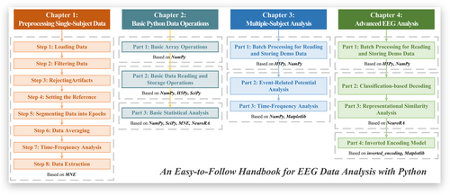
Overview of our handbook. It includes four chapters and subsections with the main packages used in the corresponding sections.
We sincerely hope that our EEG handbook offers valuable insights and suggestions. While we have endeavored to present a very easy-to-follow tutorial, it understandably cannot be directly applied to your own EEG data in its entirety. However, with some straightforward modifications, you might find yourself adeptly processing your data in no time. We hope our readers and users can apply this knowledge broadly. The content in this handbook may not delve deeply into every aspect; thus, the nuances and mysteries, techniques and philosophies, are left for you to discover through diligent practice and experience.
2.1 Preprocessing single-subject data
In this single-subject analysis, EEG preprocessing comprises eight steps: loading data, filtering data, rejecting artifacts, setting the reference, segmenting data into epochs, data averaging, time-frequency analysis, and data extraction.
2.1.1 Loading data
This step divides EEG processing into the following steps: reading raw data, checking raw data information, localizing channels, setting channel types, checking data information after modification, and visualizing raw data (see GitHub website, Chapter 1: Preprocessing Single-subject Data).
Since MATLAB-based EEGLAB is the most widely used EEG data analysis toolbox that most researchers are more familiar with, we use the classic dataset (“eeglab_data.set”) in EEGLAB as an example to teach how to use Python to deal with EEG data (source code, see GitHub website, Chapter 1).
Then, checking raw data information, localizing channels, setting channel types, and checking data information after modification can refer to the GitHub website (see Chapter 1). One can plot raw data waveforms (Figure 2) and the channel locations map (Figure 3) in Visualizing Raw Data, such as,
raw.plot(duration=5, n_channels=32, clipping=None)
raw.plot_sensors(ch_type='eeg', show_names=True)
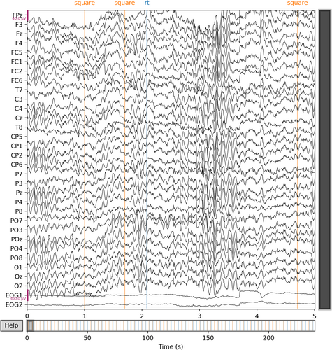
Visualization of the raw electroencephalogram data.
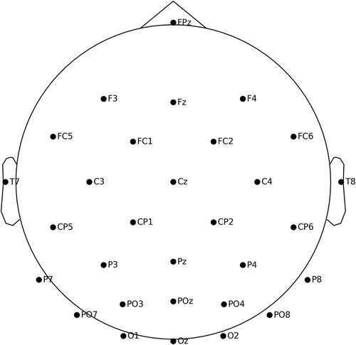
Visualization of the channel locations on the topographic map.
2.1.2 Filtering data
This step divides EEG processing into the following stages: notch filtering and high/low-pass filtering. The power spectrum in 2.1.1 shows that there might be ambient noise at around 60 Hz. Use the trap filter to remove utility frequency. Various countries and areas may have different utility frequencies. Remember to judge it by the power spectrum. In preprocessing, high-pass filtering is usually a necessary step. The most common filtering operation is a low-pass filter at 30 Hz and a high-pass filter at 0.1 Hz. High-pass filtering eliminates voltage drift, and low-pass filtering eliminates high-frequency noises (see GitHub website, Chapter 1).
2.1.3 Rejecting artifacts
This step divides EEG processing into the following steps: remove bad segments, remove bad channels, and independent components analysis (ICA). Among them, ICA includes the following steps: run ICA, plot the timing signal of each component, plot the topography of each component, check the signal difference before and after the removal of a component/several components, visualize each component, and exclude components (see GitHub website, Chapter 1).
Marking bad segments can be done manually via the MNE-Python GUI. MNE does not delete the bad segments directly. However, it marks the data with bad markers. In the subsequent data processing, we can set the parameter “reject_by_annotation” as True in functions to automatically exclude the marked segments during data processing. If you encounter the problem that the GUI window does not pop up, please add the following code to the top of the script.
MNE does not delete the bad channels directly. MNE marks them with “bad” labels. In the example below, we assume that channel “FC5” is bad. Thus, we can mark “FC5” as “bad”:
raw.info['bads'].append('FC5')
print(raw.info['bads']))
Of course, we can also add multiple bad channels (see GitHub website, Chapter 1). The programming strategy of the ICA step in MNE is to first build an ICA object (an ICA analyzer) and then use this ICA analyzer to examine the EEG data (through methods of the ICA object). Since ICA is ineffective for low-frequency data, ICA and artifact component removal are based on high-pass 1 Hz data and then applied to high-pass 0.1 Hz data. We can plot the topography of each component (Figure 4) by running
ica.plot_components ()
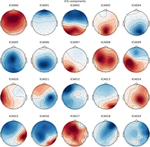
Visualization of the topographies of independent components analysis components.
For the other steps, please see GitHub website, Chapter 1: Preprocessing Single-subject Data, Step 3 Rejecting Artifacts.
2.1.4 Setting the reference
If you want to use the papillary reference method in this step, we usually choose “TP9”and “TP10” as reference channels with the following codes:
raw.set_eeg_reference(ref_channels=['TP9','TP10'])
You can use the average reference method with the following code:
raw.set_eeg_reference(ref_channels='average')
You can use the REST reference method with the following code: You must pass in a forward parameter. For details, see the corresponding MNE introduction at https://mne.tools/stable/auto_tutorials/preprocessing/55_setting_eeg_reference.html.
raw.set_eeg_reference(ref_channels='REST', forward=forward)
You can use a bipolar reference method with the following code: (“EEG X” and “EEG Y” correspond to the anode and cathode leads used for reference, respectively).
raw_bip_ref = mne.set_bipolar_reference(raw, anode=['EEG X'], cathode=['EEG Y'])
2.1.5 Segmenting data into epochs
This step divides EEG processing into the following steps: extracting event information, event information data type conversion, segmenting data, visualizing segmented data, and plotting the power spectrum topology (see GitHub website, Chapter 1).
To plot the power spectrum topology (Figure 5), we can run
bands = [(4, 8, 'Theta'), (8, 12, 'Alpha'), (12, 30, 'Beta')]
epochs.plot_psd_topomap(bands=bands, vlim='joint')

Visualization of the scalp topography of PSD for various frequency bands.
2.1.6 Data averaging
MNE uses the Epochs class to store segmented data and the Evoked class to store evoked (after averaging) data. This step divides EEG processing into the following steps: average data and visualize evoked data. The visualize evoked data step includes the following steps: plot channel-wise timing signals, plot topographic maps, plot evoked data as butterfly plot and add topographic maps, plot channel-wise hotmaps, plot 2d topography, and plot the average ERP of all channels (see GitHub website, Chapter 1).
To plot evoked data as a butterfly plot and add topographic maps (Figure 6), we can run
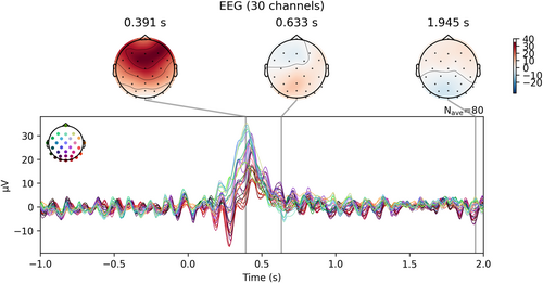
Visualization of the evoked data as a butterfly plot combined with topographic maps for several time points.
evoked.plot_joint ()
In plot 2D topography (Figure 7), we can run
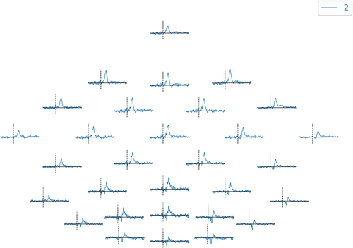
Visualization of the topographic map of the evoke data.
evoked.plot_topo ()
2.1.7 Time-frequency analysis
-
Morlet wavelets, corresponding to mne.time_frequency.tfr_morlet ()
-
DPSS tapers, corresponding to mne.time_frequency.tfr_multitaper ()
-
Stockwell Transform, corresponding to mne.time_frequency.tfr_stockwell ()
-
“mean”, to subtract the baseline mean
-
“ratio”, to divide by the baseline mean
-
“logratio”, to divide by the baseline mean and take the logarithm
-
“percentage”, to subtract the baseline mean and divide by the baseline mean
-
“zscore”, to subtract the baseline mean and divide by the baseline standard deviation
-
“zlogratio”, to divide by the baseline mean, take the logarithm, and then divide by the standard deviation of the baseline
The detailed example uses the logratio method for baseline correction. Please see GitHub website, Chapter 1: Preprocessing Single-subject Data, Step 7 Time-Frequency Analysis.
2.1.8 Data extraction
After completing the relevant calculations, we always extract the raw data array, segmented data array, and time-frequency result array, etc. In MNE, the Raw Class (raw data type), Epochs Class (segmented data type), and Evoked Class (averaged data type) provide the get_data () method. And the AverageTFR Class (time-frequency analysis data type) provides the.data attribute.
This step divides EEG processing into the following steps: use “get_data()” and use “.data” (see GitHub website, Chapter 1: Preprocessing Single-subject Data, Step 8 Data Extraction).
2.2 Basic Python data operations
According to the analytical skills used in EEG data processing, this section provides a basic tutorial on using Python to conduct array operations and statistical analysis. It includes basic array operations, basic data reading and storage operations, and basic statistical analysis.
2.2.1 Basic array operations
NumPy arrays are the most common data type for analysis operations when processing data with Python. In the first part, we will introduce some basic yet crucial NumPy array operations and their implementations in data analysis. This step divides EEG processing into the following steps: generating arrays, flattening the matrix into the vector, modifying array sizes (reshaping the array), array transposition, array merging, averaging values in an array, and converting a non-NumPy object into a NumPy array.
This handbook's operational guide is based on NumPy arrays. Therefore, users can easily perform customized analyses based on array-form EEG data.
2.2.2 Basic data reading and storage operations
This part introduces some basic operations for data (array) reading and storage based on Python. This step divides EEG processing into the following steps: data reading based on MNE, storing and reading data with h5py, storing and reading data with NumPy, storing and reading a 2-dimensional array into a text file with NumPy, reading.mat files as NumPy array. Additionally, we explain how to save NumPy array-form data as.mat files for users who want to conduct subsequent analysis with MATLAB.
2.2.3 Basic statistical analysis
This section introduces a series of basic statistical operations to conduct group analysis of EEG data from multiple subjects. Please see GitHub website, Chapter 2: Basic Python Data Operations.
2.3 Multiple-subject analysis
The section on multisubject analysis comprises the following three parts: batch processing for reading and storing demo data, ERP analysis, and time-frequency analysis.
2.3.1 Batch processing for reading and storing demo data
This step divides EEG processing into the following steps: preprocessed demo data 1 and batch processing for reading demo data 1 and saving it as a.h5 file.
The original dataset is based on the article “A multi-subject, multi-modal human neuroimaging dataset” by Wakeman & Henson, published in Scientific Data in 2015.6 In this experiment, there are three categories of faces: familiar faces, unfamiliar faces, and scrambled faces, with 150 images for each type, totaling 450 stimulus images. Participants wore an EEG cap to perform a simple perceptual task, which included an unpredictable stimulus phase of 800–1000 ms, a delay of 1700 ms, and an inter-trial interval (ITI) of 400–600 ms. Each image was viewed twice, with 50% of the stimulus images being presented immediately after the first viewing, while the other 50% appeared several other trials after the first viewing. Here, we extracted only the EEG data from the first eight subjects who viewed multiple familiar face images for the first time and then immediately viewed some of these images again in the following trial.
Taking sub1 as an example, “sub1_first.mat” contains EEG data for the first viewing of familiar face images, and “sub1_rep.mat” contains EEG data for the immediate second viewing of familiar faces. The number of trials in the former case was double that in the latter. We preprocessed (0.1–30 Hz filtering) and segmented the data. The data includes 74 channels (of which 70 are EEG channels, with channels 61, 62, 63, and 64 being eye movement channels) and a sampling rate of 250 Hz. Each trial covers for 0.5 s before to 1.5 s after the stimulus presentation, with 500 time points per trial.
2.3.2 Event-related potential analysis
Using Demo Data 1 as an example, we visualize the ERP results and conduct statistical analyses for two conditions in the experiment: the first viewing of familiar faces and the immediate repeated viewing of familiar faces. This step divides EEG processing into the following steps: read data and average epochs, and statistical analyses and visualization (see GitHub website, Chapter 3: Multiple-Subject Analysis).
In statistical analyses and visualization, we can plot the joint ERP results under two conditions (Figure 8),
plot_erp_2cons_results(erp_first, erp_rep, times, con_labels=['First', 'Repetition'], p_threshold=0.05, labelpad=25)
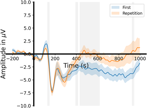
Visualization of the joint event-related potential results under both the first viewing and the immediate repeated viewing of familiar face conditions.
2.3.3 Time-frequency analysis
We will visualize the time-frequency results and conduct statistical analyses for two conditions in the experiment: the first viewing of familiar faces and the immediate repeated viewing of familiar faces. This step divides EEG processing into the following steps: read data and conduct the time-frequency analysis and statistical analyses and visualization (see GitHub website, Chapter 3).
In statistical analyses and visualization, we plotted the time-frequency result under the condition of the first viewing of familiar faces (Figure 9),
freqs = np.arange(4, 32, 2)
times = np.arange(-200, 1000, 4)
plot_tfr_results(tfr_first_No50, freqs, times, p=0.05, clusterp=0.05, clim=[-3, 3])
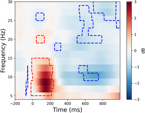
Visualization of the time-frequency results under the condition of the first viewing of familiar faces.
Please see GitHub website, Chapter 3: Multiple-Subject Analysis for the other steps.
2.4 Advanced EEG analysis
The section on advanced EEG analysis comprises the following four parts: batch processing for reading and storing demo data, classification-based decoding,8, 15-17 RSA,5, 9, 10, 18, 19 and IEM14, 20, 21 (see GitHub website, Chapter 4: Advanced EEG Analysis).
2.4.1 Batch processing for reading and storing demo data
This step divides EEG processing into the following steps: preprocessed demo data 2 and batch processing for reading demo data 2 and saving it as a.h5 file (see GitHub website, Chapter 4).
In preprocessed demo data 2, the original dataset is based on the data from Experiment 2 in the article “Dissociable Decoding of Spatial Attention and Working Memory from EEG Oscillations and Sustained Potentials” by Bae & Luck, published in the Journal of Neuroscience in 2019.15 It involves a visual working memory task that requires participants to remember the orientation of a teardrop shape presented for 200 ms. After a delay of 1300 milliseconds, it presented a teardrop shape with a random orientation, and participants were required to rotate the mouse to align its orientation as closely as possible with their recollection. The stimulus could appear in 16 orientations and 16 locations. Here, only data from the first five participants are extracted, consisting of preprocessed ERP data (see the original article for preprocessing parameters) with labels for each trial's orientation and location.
2.4.2 Classification-based decoding
This step divides EEG processing into the following steps: get EEG data and labels, time-by-time EEG decoding, and cross-temporal EEG decoding (see GitHub website, Chapter 4).
In time-by-time EEG decoding, we can plot time-by-time orientation decoding results (Figure 10),
plot_tbyt_decoding_acc(accs_ori, start_time=-0.5, end_time=1.5, time_interval=0.02, chance=0.0625, p=0.05, cbpt=True, stats_time=[0, 1.5], xlim=[-0.5, 1.5], ylim=[0.05, 0.15])
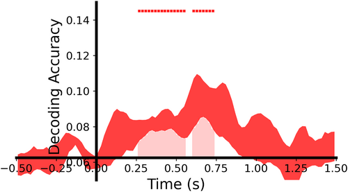
Visualization of the time-by-time orientation decoding results.
In cross-temporal EEG decoding, we can plot cross-temporal orientation and position decoding results (Figure 11),
plot_ct_decoding_acc(accs_crosstime_ori, start_timex=-0.5, end_timex=1.5, start_timey=-0.5, end_timey=1.5, time_intervalx=0.02, time_intervaly=0.02, chance=0.0625, p=0.05, cbpt=True, stats_timex=[0, 1.5], stats_timey=[0, 1.5], xlim=[-0.5, 1.5], ylim=[-0.5, 1.5], clim=[0.06, 0.075])
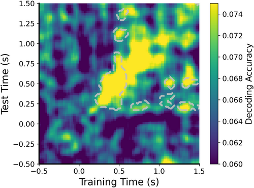
Visualization of the cross-temporal orientation decoding results.
2.4.3 Representational similarity analysis
This step divides EEG processing into the following steps: calculate EEG representational dissimilarity matrices (RDMs), construct the hypothesis-based RDM, and RSA (see GitHub website, Chapter 4: Advanced EEG Analysis).
2.4.4 Inverted encoding model
This step divides EEG processing into the following steps: Apply an enhanced inverted encoding model (eIEM) to decode orientation information, define a function to plot eIEM results, and apply eIEM to decode position information (see GitHub website, Chapter 4: Advanced EEG Analysis).
In this part, we refer to a preprint “Scotti, P. S., Chen, J., & Golomb, J. D. (2021). An eIEM for neural reconstructions. bioRxiv”14 that utilized an eIEM.
3 DISCUSSION AND CONCLUSION
This EEG handbook demonstrates the efficacy of Python libraries, such as MNE-Python and NeuroRA, in streamlining the EEG data preprocessing and analysis process, providing an easy-to-follow guide for EEG researchers in cognitive neuroscience and related fields. Since our handbook focuses on using Python to begin analyzing EEG data, we have not included an extensive introduction to the theoretical aspects, such as understanding the principles behind the phenomena of EEG data, the mathematical foundations of various analysis methods, and interpreting their results. We hope that everyone will learn how to conduct these analyses and understand why they should be done by exploring more literature. Moreover, our handbook still lacks coverage of many topics that may be of interest, such as brain connectivity analysis based on resting-state EEG,22-24 image reconstruction from EEG data,25-29 and research combining artificial neural networks with EEG data.16, 17, 30-32 We will add more content to the handbook to make this tutorial more comprehensive. We encourage users to suggest new analysis methods and algorithms via email or by submitting Issues via our GitHub project page.
This handbook is a pivotal contribution to helping researchers conduct EEG data analysis, offering a clear, step-by-step guide that demystifies complex analytical processes, thereby empowering researchers to conduct more in-depth and insightful EEG studies. At the same time, we also hope that more people will join the open-source community in cognitive neuroscience. With the strong advocacy for open science and the rapid innovation in various research methods in psychology and neuroscience, we need more effective learning guides and shared resources to drive continuous progress in the field.
AUTHOR CONTRIBUTIONS
Zitong Lu: Conceptualization; formal analysis; investigation; methodology; project administration; visualization; writing – original draft; writing – review & editing. Wanru Li: Conceptualization; formal analysis; methodology; validation; writing – review & editing. Lu Nie: Conceptualization; formal analysis; methodology; validation; writing – review & editing. Kuangshi Zhao: Conceptualization; formal analysis; methodology; validation; writing – review & editing.
ACKNOWLEDGMENTS
This study was financially supported by the National Social Science Fund of China (23CYY048). We express our sincere gratitude for the active support and feedback from the members of the WeChat groups “MNE-Python Study” and “NeuroRA Q&A”. We are particularly thankful for the valuable reference provided by Steven Luck's book An Introduction to the ERP Technique and the official documentation and tutorials from EEGLab and MNE-Python. Special thanks go to Mengxin Ran, an undergraduate from OSU Vision & Cognitive Neuroscience Lab, for her meticulous review of the content. We are grateful to the authors of the public datasets used in this tutorial, including Daniel Wakeman, Richard Henson, Gi-Yeul Bae, and Steven Luck, who significantly contributed to the open science community. These datasets form the foundation for our handbook's detailed examples. We thank all the readers who helped promote our handbook and provided support and feedback after the first Chinese version 3 years ago.
CONFLICT OF INTEREST STATEMENT
Although Kuangshi Zhao is currently employed by Neuracle Technology (CHangzhou) Co Ltd, there are no conflicts of interest regarding his involvement in this paper and his work at the company. The other authors declare that they have no conflicts of interest.
ETHICS STATEMENT
Ethics approval was not needed in this study.
Open Research
DATA AVAILABILITY STATEMENT
The data that support the findings of this study are available on GitHub: https://github.com/ZitongLu1996/Python-EEG-Handbook and https://github.com/ZitongLu1996/Python-EEG-Handbook-CN.


