Volume 2014, Issue 1 505890

Research Article

Open Access

Retrofitting Transportation Network Using a Fuzzy Random Multiobjective Bilevel Model to Hedge against Seismic Risk

Lu Gan,

Lu Gan

Urban and Rural Development College, Sichuan Agricultural University, Dujiangyan 611830, China sicau.edu.cn

Uncertainty Decision-Making Laboratory, Sichuan University, Chengdu 610064, China scu.edu.cn

Search for more papers by this author

Jiuping Xu,

Corresponding Author

Jiuping Xu

[email protected]

Uncertainty Decision-Making Laboratory, Sichuan University, Chengdu 610064, China scu.edu.cn

State Key laboratory of Hydraulics and Mountain River Engineering, Sichuan University, Chengdu 610064, China scu.edu.cn

Search for more papers by this author

Lu Gan,

Lu Gan

Urban and Rural Development College, Sichuan Agricultural University, Dujiangyan 611830, China sicau.edu.cn

Uncertainty Decision-Making Laboratory, Sichuan University, Chengdu 610064, China scu.edu.cn

Search for more papers by this author

Jiuping Xu,

Corresponding Author

Jiuping Xu

[email protected]

Uncertainty Decision-Making Laboratory, Sichuan University, Chengdu 610064, China scu.edu.cn

State Key laboratory of Hydraulics and Mountain River Engineering, Sichuan University, Chengdu 610064, China scu.edu.cn

Search for more papers by this author

First published: 12 January 2014

https://doi.org/10.1155/2014/505890

Citations: 4

Academic Editor: Mohamed Fathy El-Amin

Share a link

Email
Wechat
Bluesky

Abstract

This paper focuses on the problem of hedging against seismic risk through the retrofit of transportation systems in large-scale construction projects (LSCP). A fuzzy random multiobjective bilevel programming model is formulated with the objectives of the retrofit costs and the benefits on two separate levels. After establishing the model, a fuzzy random variable transformation approach and fuzzy variable approximation decomposition are used to deal with the uncertainty. An approximation decomposition-based multi-objective AGLNPSO is developed to solve the model. The results of a case study validate the efficiency of the proposed approach.

1. Introduction

Transportation networks play a very important role in both urban and rural areas, as well as in industrial sites such as large-scale construction sites. Liu et al. [1] stated that transportation networks are critical infrastructure and their smooth operation is important for maintaining the normal functions of society. However, disasters, especially earthquakes, cause not only tremendous economic losses and social chaos but also enormous damage to infrastructure (e.g., 2008 Wenchuan Earthquake, 2010 Chile Earthquake, and 2011 Japan Earthquake). Thus, as Liu et al. [1] pointed out, seismic risk control should also consider the effect that damaged or destroyed transportation networks have on the effectiveness of postdisaster rescue and repair activities and the associated socioeconomic losses. Under a seismic risk threat, retrofit decisions are considered to be an effective protective measure and can have a significant impact on these systems [1–3]. Therefore, promoting retrofit decisions for transportation networks is necessary to hedge against seismic risk.

The research in this area has mainly focused on the retrofitting of bridges for transportation networks [4–6]. Werner et al. [2] extended seismic retrofits to highway systems. Afterwards, Liu et al. [1] established a two-stage stochastic programming model for retrofit decisions for transportation network protection. This previous research, however, has primarily focused on urban transportation, but it is essential that transportation networks in large-scale construction projects (LSCP) also be considered. As a critical infrastructure, the smooth operation of these networks is important for maintaining the normal progress of these projects. Therefore, it is necessary to control the seismic risk for LSCP transportation networks to mitigate losses. When considering LSCP transportation network retrofits, there are significant challenges. First, these transportation systems have not only permanent links and temporary links to consider but must also assess the critical links (i.e., bridge, tunnel, etc.) and the noncritical links. Secondly, the retrofit decision making environment is a mutual environment involving an investor who pays for the retrofit and an administrator who controls the transportation systems. Thirdly, a consideration of the environmental costs for the investor has increasingly become necessary for social and economic development. Lastly, a majority of the previous research has assumed that seismic damage is classified into five categories and there is a set of discrete probabilities associated with each of the five damage categories. In practice, however, the situation is often not that simple, and the description of the possible result of seismic damage is vague and uncertain. In this case, this needs to be qualified with a vague perception of a crisp but unobservable random variable. Hence, due to the complexity of assessing the seismic risk to property, seismic damage is subject to uncertainty with both fuzziness and randomness, that is, fuzzy random in nature. More recently, since Kwakernaak [7] proposed the concept of the fuzzy random variable, considerable research has been done, which has allowed for its application in many areas [7–13]. Unfortunately, there has been little research which has discussed a mixture of fuzziness and randomness in a transportation network retrofit problem. Therefore, the uncertainty with hybrid fuzziness and randomness induced by the seismic damage risk to property needs to be further studied and elaborated.

The fuzzy random variable was proposed by Kwakernaak [7] who regarded it as “random variables whose values are not real, but fuzzy numbers.” From another view, Puri and Ralescu [14] and Klement et al. [15] regarded a fuzzy random variable as a random fuzzy set. Fuzzy random variables represent a well-formalized concept which has underlain many recent probabilistic and statistical studies involving data obtained from a random experiment when these data are assumed to be fuzzy set valued [16]. Therefore, in a transportation network retrofit problem, the description of seismic damage is considered a fuzzy random variable, that is, a discrete distribution variable with a vague perception (i.e., triangular fuzzy number). Several research works have demonstrated how these fuzzy random coefficients can be converted into crisp values. Usually, at first, the fuzzy random variables are transformed into fuzzy numbers using the fuzzy expected values [17] or transformed into (α₁, σ)-level trapezoidal fuzzy variables through an approach proposed in Xu and Liu [12]. Then, these fuzzy numbers are transformed into deterministic values using their expected value [18] or (α, β)-satisfactory solution to the programming is determined using fuzzy coefficients [12]. In this case, based on the properties of the fuzzy random seismic damage in this study, the theorem and the proof presented in Xu and Liu [12] are adjusted to allow for a discrete random distribution to obtain the equivalent fuzzy bilevel programming model. Then, using the theorem proposed by Zhang et al. [19], decomposition is used on these fuzzy variables to derive an approximate solution to the model.

Under these emerging challenges, this paper formulates a fuzzy random multiobjective bilevel programming model for a transportation network retrofit decision to hedge against seismic risk in an LSCP. The distinctions in the link types allow for the recognition of the retrofit and reconstruction costs. The investor and the administrator are the decision-makers on two separate levels. Retrofit costs which include the environmental costs and the retrofit benefits are the two objectives of the investor, and the retrofit benefits are the objective of the administrator. In order to describe the hybrid uncertainty of possible seismic damage, fuzzy random variables are introduced in the programming model, the use of which has been applied in many areas [10, 18]. To cope with the proposed fuzzy random multiobjective bilevel programming model, a transformation approach is used to obtain an equivalent fuzzy bilevel programming model. This approach transforms the fuzzy random variables in the model into fuzzy variables which are similar to trapezoidal fuzzy variables. Then, decomposition is utilized on these fuzzy variables using a fuzzy number decomposition theorem [19]. To solve the model, an approximation decomposition-based multiobjective AGLNPSO is developed in this paper. Through the decomposition of the fuzzy variables, the models are successively solved until termination, and the approximation solutions are obtained. The multiobjective AGLNPSO is a combination of the Pareto Archived Evolution Strategy (PAES) [20] and the AGLNPSO [21] which is developed by incorporating an adaptive particle swarm optimization (APSO) [22] with a GNLPSO [23] and a multiple objectives particle swarm optimization (MOPSO) [24].

This study contributes to the literature by adopting the work of Liu et al. [1] to an LSCP and describing the complex uncertain seismic damage scenario using fuzzy random variables. Bilevel decisions involving the investor and the administrator, distinctions between the various link types, and the specification of the retrofit decisions into several ranks according to the seismic damage scenario provide a more reasonable and practical description of the problem. The consideration of the environmental costs in the transportation network in an LSCP enhances the focus for management. To the best of our knowledge, an integrated approach to deal with fuzzy random variables has not been previously comprehensively studied. The approximation decomposition-based multiobjective AGLNPSO is developed as a useful tool to solve the problem, in which both the bilevel and multiobjective environments are considered.

The remainder of this paper is as follows. The problem description, the fuzzy random multiobjective bilevel programming model, the transformation approach, and the approximation decomposition are given in Section 2. An approximation decomposition-based multiobjective AGLNPSO is developed in Section 3. A case study is presented in Section 4. Finally, advantages, limitations, and possible future extensions of this work are presented in Section 5.

2. Modeling

In this section, the concepts for the LSCP transportation network, the bilevel decision framework, the environmental costs, and the fuzzy random seismic damage scenario are introduced. A multiobjective bilevel programming model for the problem considering fuzziness and randomness is established. See in the following the notations used to describe the model.

Index

a: Link in transportation network, a ∈ A
b Node in transportation network, b ∈ B
v Variable environment cost, v ∈ V
f Fixed environmental cost, f ∈ F
i Retrofit output, i ∈ I
j Retrofit activity, j ∈ J
k Origin-destination pair considered as commodity, k ∈ {1, …, K}.

Variables

: Increased variable retrofit costs for permanent link by basic rank (i.e., rank 1)
: Variable retrofit costs for temporary link by basic rank (i.e., rank 1)
: Increased fixed retrofit costs for permanent link
: Fixed retrofit costs for temporary link
ρ: Weight of environmental costs
: Increased variable environmental costs for permanent link by basic rank (i.e., rank 1)
: Variable environmental costs for temporary link by basic rank (i.e., rank 1)
: Fixed environmental costs
: Percent of activity cost center j in variable environment cost v
: Percent of output i in fixed environment cost f
: Variable environmental costs of activity cost center j
am_j: Cost of driver at activity cost center j
ra_j: Driver rate at activity cost center j
am_ij: Cost of driver for output i in activity cost center j
C: Retrofit costs including environmental costs
Q: Retrofit benefits
: Preretrofit link damage state for link a
: Postretrofit link damage state for link a
: Increased variable reconstruction cost for permanent link by basic rank (i.e., rank 1)
: Variable reconstruction cost for temporary link by basic rank (i.e., rank 1)
: Increased fixed reconstruction cost for permanent link
: Fixed reconstruction cost for temporary link
γ: Weight coefficient conversion time to monetary value
: Free flow travel time and link a
α: Coefficient of BPR function
fl_a: The total flow on link a
: Practical capacity of link a is set at 90% of the design capacity
β: BPR function coefficient
ca_b: Capacity of node b
W: Node-commodity adjacency matrix
M: Link-commodity adjacency matrix.

Decision Variables

(1)

2.1. LSCP Transportation Network

The LSCP transportation network is composed of an internal road system and an external road system and is always built based on the existing links around the site which are connected with the newly built links according to transportation need. There are two types of links (i.e., permanent links and temporary links) which vary considerably in terms of quality. In addition, according to the different functions, the links are divided into critical links and noncritical links. Critical links are those which have vital transport functions such as bridges and tunnels and which should be preferentially taken into account [1]. The retrofit decisions for the different link types vary. That is, the links being considered for the retrofit are either considered to be permanent or critical. The retrofit and reconstruction costs for the temporary links are lower than those for the permanent links. Further, the retrofit decision is specific with 0 (i.e., no retrofit) and there are several ranks according to the seismic damage scenarios.

2.2. Bilevel Decision Framework

In this paper, the seismic hazard retrofit decision for an LSCP transportation network involves two participants (i.e., the investor who pays for the retrofit and the administrator who controls the transportation). Therefore, these two participants are the decision-makers on two levels, both of whom successively make the retrofit decisions. The investor on upper level decides which retrofit rank should be taken for each link within the range and, therefore, the two objectives on this level are the retrofit costs including the environmental costs and the retrofit benefits. The administrator decides on the commodity flow (i.e., the transportation network flow once seismic damage has occurred) on the lower level according to the decision results of the upper level. On this level, the retrofit benefits are the primary objective. In this paper, the retrofit benefits are quantified as reconstruction and travel delay cost savings. The investor on the upper level affects the decisions of the administrator on lower level, but does not fully control them. The administrator makes their decision autonomously based on the scope of the decision of the upper level.

2.3. Environmental Costs

In recent years, more attention has been paid to environmental problems as these have begun to seriously affect both local communities and the economy. Thus, it is essential to consider the environmental costs in the LSCP. In addition, as environmental costs affect the overall project cost, it is necessary to effectively record and calculate environmental costs in the LSCP. Generally, many environmental costs are not usually tracked systematically or attributed to the related processes and outputs but are simply summed and added to total cost [25]. The fact that environmental costs are not fully recorded often leads to distorted calculations [25]. Activity based costing (ABC) is an effective method to record and calculate environmental costs [26]. Cooper provided a comprehensive discussion of ABC [27–30], following the pioneering work of [31, 32]. This method treats activities as accounting objects, and identifies and measures the amount of activities using cost drivers.

The environmental costs for retrofitting LSCP transportation networks based on the ABC are as shown in Figure 1. As can be seen, the environmental costs are fully recorded according to the environmental cost categories proposed in [25]. Note that some environmental cost categories are related to the work processes, and others are not. Then, all the outputs involved in retrofitting the LSCP transportation network are determined and an analysis of the activity processes and a definition of the activities are prepared to determine the environmental costs. Every activity corresponds to an activity cost center. Jasch [25] proposed that the costs should be more precisely allocated to cost centers. Therefore, environmental costs are either directly allocated to each activity cost center or systematically traced to the responsible environmental media. Of course, if those costs are attributed to outputs directly (i.e., they are not related to the work processes), it is not necessary to allocate them to activity cost centers. Then, the cost drivers for the activity cost centers are determined and the cost driver amounts measured to calculate the cost driver rates. Finally, the environmental costs of each output are determined.

Details are in the caption following the image — **Figure 1**
Open in figure viewer PowerPoint

Obtain environmental costs for retrofitting transportation network in LSCP based on ABC.

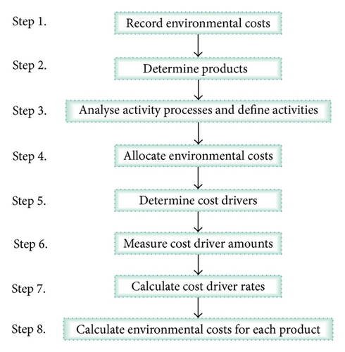
Therefore, by using a complete recording method, distortion in the environmental costs can be avoided and through this precise allocation it is easier to effectively manage these costs as it is possible to systematically trace them to the related processes and outputs.

2.4. Fuzzy Random Seismic Damage Scenario

To better understand the concepts for the fuzzy random seismic damage scenario, this subsection gives some basic knowledge for the definition and properties of the fuzzy random variables. After Zadeh [33] proposed the concept of fuzzy sets, many scholars have usually tied fuzziness to randomness as possible random outcomes have to be described using fuzzy sets. To describe this fuzziness and randomness, Kwakernaak [7] proposed the concept of fuzzy random variables in 1978. Kruse and Meyer [17] then worked on an expanded version of a similar model. In addition, Puri and Ralescu [14] and Klement et al. [15] also defined fuzzy random variables from other angles. In this paper, the fuzzy random variables are defined in the real number set. This makes the above definitions equivalent [34]. Here, the definition proposed by [14] is utilized.

In the following, ℝ is denoted as the set of all real numbers, ℱ_c(ℝ) is denoted as the set of all fuzzy variables, and 𝒦_c(ℝ) is denoted as all of the nonempty bounded close intervals.

Definition 1 (see [14].)In a given probability space (Ω, 𝒜, Pr), a mapping is called a fuzzy random variable in (Ω, 𝒜, Pr); if α ∈ (0,1], the set-valued function ,

(2)

is ℱ measurable.

Definition 2 (see [35].)If are fuzzy random variables defined in the probability space on (Ω, 𝒜, Pr), then is called fuzzy random vector.

Lemma 3 (see [36].)Let be a fuzzy random vector, and let f be a continuous function from ℝ^𝕞 to ℝ. Then is a fuzzy random variable.

Definition 4 (see [14].)In a given probability space (Ω, 𝒜, Pr), if ω ∈ Ω, α ∈ [0,1], the mapping and are integrable; then is called the integrated bounded fuzzy random variable on the probability space (Ω, 𝒜, Pr).

Definition 5 (see [14].)Let be an integrated bounded fuzzy random variable on the probability space (Ω, 𝒜, Pr); the expected value of is defined as the only fuzzy set in ℝ; for all α ∈ [0,1], it satisfies

(3)

where

is the Aumann integral of

about P and L¹(P) denote all of the integrable function f : Ω → ℝ about the probability measure P.

Lemma 6 (see [37].)Let (Ω, 𝒜, Pr) be complete probability space; is an integrated bounded fuzzy random variable. Then for all α ∈ [0,1], the α-set of is the compact convex interval as follows:

(4)

Lemma 7. Let (Ω, 𝒜, Pr) be complete probability space; , are integrated bounded fuzzy random variables on (Ω, 𝒜, Pr), λ, γ ∈ ℝ, and then

(5)

For the fuzzy random seismic damage scenario, according to [1], advanced structural analysis can lead to a probabilistic assessment of the structural damage for a given earthquake, in terms of a set of discrete probabilities associated with each of the five damage categories. Seismologists also have made predictions as to the probabilities of various earthquake occurrences. These two sets of probabilistic estimations from earthquake-structural engineers and seismologists can be combined to prepare the damage prediction [1]. For the convenience of discussion, seismic damage to a structure (i.e., LSCP transportation network) is usually classified into five categories ranging from no damage to complete collapse. However, a description of the perception result for seismic damage is a category which is vague. In this case, a vague perception of a crisp but unobservable random variable is used as in the following:

(6)

Therefore, the seismic damage scenario can be viewed as a fuzzy random variable, which has a similar sense to the minor automobile collision damage outlined in [10]. See Figure 2 for a detailed description.

An example can be used to explain how to use the fuzzy random variable and to describe the uncertainty in a seismic damage scenario. Suppose that there is a link a ∈ A in an LSCP transportation network. Seismic damage perception has five categories 1, 2, 3, 4, and 5 ranging from no damage to complete collapse and seismic damage randomly emerges with a certain probability. On the other hand, the description of the perception result is vague with values such as “about 1” and “about 3.” These denote the fuzzy sets and can be conveniently described using triangular fuzzy sets, as shown in Figure 3. Here it is assumed that the probabilities for the five categories are 0.1, 0.2, 0.3, 0.3, and 0.1, so the seismic damage scenario can be seen as a fuzzy random variable as in (7) and as shown in Figure 3. It should be mentioned that one damage scenario has different meanings for the different damage ranks (i.e., its membership is different for each different damage rank). Similar examples can be found in [10]. Consider

(7)

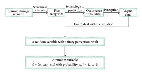
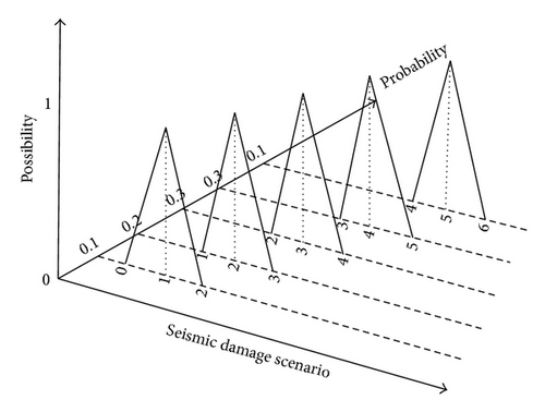
It should be noted that the same category may have different possibilities for different links.

2.5. Model Formulation

Denote a transportation network as G(B, A), where B is the set of nodes and A is the set of network links. The decision variable on the upper level is u_a ∈ {0,1, 2,3, 4,5}, which means that a decision has been done for link a to be retrofitted at rank u_a, a ∈ A. For each commodity k ∈ {1, …, K}, x_k ∈ R₊ is the commodity flow (i.e., the decision variable on the lower level), and ca_b ∈ R₊ is the capacity of node b. Denote fl_a as the total flow on link a (i.e., fl_a = Mx, for all a ∈ A). To model the retrofit decision with seismic risk in this paper, the assumptions are as follows.

(1)
The LSCP transportation network is composed of internal road systems and external road systems and has two types of links, permanent and temporary. In addition, two types of links are designated as critical or noncritical links.
(2)
The links under retrofit consideration are those which are either permanent or critical.
(3)
The retrofit activity process is the same for both permanent and temporary links.
(4)
In the retrofit, the variable environmental and reconstruction costs for the temporary links are considered of less importance than the permanent links.
(5)
The retrofit costs and the retrofit decision have a linear relationship which can be easily relaxed without changing the structure of the proposed model, as long as the data are available to support a more detailed analysis.
(6)
The variable environmental costs and the retrofit decision have a linear relationship which can be easily relaxed without changing the structure of the proposed model, as long as the data are available to support a more detailed analysis.
(7)
Origin-destination pairs (i.e., commodities) are determined in advance.
(8)
Traffic flow can be controlled to achieve system equilibrium [1].
(9)
The preretrofit link damage state is defined as the seismic damage scenario minus the retrofit decision u_a developed from [1].
(10)
Reconstruction costs have a linear function with the postretrofit damage state which can be easily relaxed without changing the structure of the proposed model.

2.5.1. Upper-Level Programming

The investor on the upper level makes a decision as to whether there should be a retrofit for each link a in the transportation network and what rank the retrofit should be. The decision needs to fully consider the link types (i.e., permanent and temporary, critical and noncritical).

Objective Functions. One objective on the upper level is to minimize the retrofit costs, which include the environmental costs. In this paper, from a systems view, the retrofit costs are added directly to the objective function, which differs from [1]. The investor aims to minimize costs through their decision. Based on this assumption, the retrofit costs can be calculated using the sum of the variable and fixed costs for all links in the network. The retrofit costs for the temporary links are lower than the permanent links. In order to distinguish link types, 0-1 variables are introduced. m_a with 1 indicates a permanent link and is 0 otherwise; n_a with 1 indicates a critical link and is 0 otherwise. Therefore, the retrofit costs can be denoted as . Here, ∨ is defined as max , namely, max [m_a, n_a].

Based on the ABC described above and the assumptions,

is the variable environment cost v and

denotes the fixed environmental cost f. Through an analysis of the activity processes, the activity definitions, and the cost allocations,

is the variable environmental costs of activity cost center j and

is the fixed environmental costs of output i. After determining the cost drivers for the activity cost centers and measuring the cost driver amounts,

is the cost driver rate for activity cost center j. The variable environmental costs for output i are

. After this, the environmental costs can then be presented as

. Thus, the objective can be described as

(8)

Here, ρ denotes the weight of the environmental costs and is determined by the investor.

The maximization of the retrofit benefit is another upper-level objective. The decision result of the lower-level is denoted

and quantified as savings in reconstruction and travel delay costs. u is the vector of u_a, a ∈ A, and

is the vector of

. This can be described as

(9)

Here, maximizing the retrofit benefit while minimizing reconstruction costs and travel time delay is denoted as , which will be described in detail in the objective for the lower level.

Logical Constraints. To describe the discrete decision variables for practical sense, the constraints in the following are presented:

(10)

The objective functions and constraints above make up the upper-level programming with lower-level programming as in the following:

(11)

2.5.2. Lower-Level Programming

The administrator on the lower level decides on the commodity flow x_k. In transportation network literature, the flow between each origin-destination pair is often considered as one commodity. Different commodities represent travel between different origin-destination pairs. x_k is used to express the flow of k commodity. This optimal commodity flow decision seeks to achieve optimal retrofit benefits under a postretrofit state once an earthquake event has occurred and seismic damage sustained. First, it is necessary to introduce the postretrofit damage state before describing in detail the lower-level programming.

Postretrofit Damage State. A fuzzy random vector

is introduced to describe the damage to the link once an earthquake has occurred after the retrofit, which has been developed from [1]. Here,

is the vector for

. Assume that if a link is retrofitted at any rank, its damaged state (i.e., postretrofit damaged state in the earthquake) is denoted as a seismic damage scenario (i.e., preretrofit link damage state) minus the retrofit rank. Here, for demonstration, a negative postretrofit damaged state is not considered, so the negative state is treated as 0 indicating that the link will be intact. The relationship between the preretrofit link damage state

, the retrofit decision u_a, and the postretrofit damage state

is described as in the following:

(12)

For any scenario, the postretrofit damaged state of link a can describe the current damaged state of link a in an earthquake after a retrofit. Based on the above, the discussion for the lower-level programming is as follows.

Objective Function. Retrofit benefits are the objective of the administrator. They are only quantified as savings in the minimization of reconstruction and travel delay costs [1]. To maximize benefits is to minimize costs. According to this assumption, the reconstruction costs can be presented as

. This is calculated using the sum of the variable and fixed costs for all the links in the network when links are damaged in an earthquake and need to be reconstructed. Travel delay costs are the total travel time of all the links in the network. The travel time of each link is the product of link travel time and link flow. The link travel time depends on the link flow. Their relationship is usually described using a nondecreasing function such as the bureau of public roads (BPR) function [1]. The BPR function is in the form of

. Where

and fl_a are free flow travel time and flow for link a, respectively,

is the “practical capacity” of link a and is set to be 90% of the design capacity. Thus, the travel delay costs of a can be denoted as

. The objective function is presented as shown below:

(13)

where γ is a weight coefficient converting the time to a monetary value, α, β are coefficients of the BPR function, and

is as

Node Capacity Constraint. Logistics in large scale postdisaster relief is very important [38]. Therefore, once an earthquake event occurs, a working transportation network for disaster relief and the LSCP are critically important, so the nodes in the network should be fully functioning. Therefore, the node capacity should be at capacity. The constraint is to keep transport in accordance with the flow and the capacity of node b as shown in the following:

(14)

where W represents the node-commodity adjacency matrix. x is the commodity flow vector for x_k, k ∈ K. ca_b ∈ R₊ is the capacity of node b.

Flow Equation Constraint. The total flow on each link a is the sum of all flows of all commodity k that contains a and is obtained using the link commodity adjacency matrix and the commodity flow vector x as in the following:

(15)

Damaged Link Flow Constraint. This constraint restricts the link flow when a link is damaged by the earthquake as in (16). This constraint is applied to the postretrofit damaged state and the “practical capacity” of link a, which is set at 90% of the design capacity:

(16)

where fl_a is obtained in (15).

Logical Constraints. In order to describe the nonnegative variables in the model, the constraints in the following are presented:

(17)

The objective function and constraints above compose the lower-level programming as in the following:

(18)

2.5.3. Fuzzy Random Multiobjective Bilevel Programming Model

The complete multiobjective bilevel programming model under a fuzzy random environment is formulated based on the previous discussion as in the following model:

(19)

2.6. Transformation Approach for Fuzzy Random Variables

In this subsection, some basic knowledge for the fuzzy random variables is stated.

Definition 8 (see [33].)Given a domain U, if is a fuzzy set on U, then for any x ∈ U, see the following:

(20)

where

is called a membership function of x with respect to

and

denoted the grade to each point in U with a real number in the interval [0,1] that represents the grade of membership of x in

is called a fuzzy set and described as follows:

(21)

Definition 9 (see [33].)Let there be a domain U. Let be a fuzzy set which is defined on U. If α is possibility level and 0 ≤ α ≤ 1, consists of all elements whose degrees of membership in are greater than or equal to α as in the following:

(22)

then

is called the α-level set of fuzzy set

Definition 10 (see [39].)Let Θ be a nonempty set, and let P(Θ) be the power set of Θ. For each A⊆P(Θ), there is nonnegative number Pos{A}, called its possibility, such that

(1)
Pos(∅) = 0 and Pos(Θ) = 1,
(2)
Pos(⋃_k A_k) = sup _kPos(A_k) for any arbitrary collection {A_k} in P(Θ).

The triple (Θ, P(Θ), Pos) is called a possibility space. The function Pos is referred to as a possibility measure.

Definition 11 (see [40].)A fuzzy variable is defined as a function from the possibility space (Θ, P(Θ), Pos) to the real number ℝ.

Definition 12. Let ε be a discrete random variable defined on a probability space (Ω, 𝒜, Pr) with the discrete distribution P_ε(x) = P{x = x_n}, n = 1,2, …, and let θ be any given probability level and 0 ≤ θ ≤ max P_ε(x). ε_θ consists of all elements whose value of P_ε(x) for ε is greater than or equal to θ as the following:

(23)

then ε_θ is called the θ-level set of random variable ε.

As stated in Section 2.4, the definition proposed by [14] is used in this paper. Although there are many properties and transformation approaches for the fuzzy random variable, to conveniently convert programming with fuzzy random coefficients into crisp values, Xu and Liu [12] proposed a theorem which could transform fuzzy random variables into fuzzy variables similar to trapezoidal fuzzy numbers. In this paper, this theorem and proof are adjusted to a discrete random distribution with fluctuating lower, central, and upper parameters for the fuzzy properties and extended bounds of possibility for the fuzzy variable.

Theorem 13. Let

(24)

be a fuzzy random variable, which has discrete random distribution with fluctuating lower, central, and upper parameter for fuzzy property. The discrete distribution is P_ψ(x). δ is any given probability level of random variable; η is any given possibility level of fuzzy variable; then the fuzzy random variable can be transformed into a (δ, η)-level trapezoidal fuzzy variable.

Proof. Let

(25)

be a fuzzy random variable, which has discrete random distribution with fluctuating lower, central, and upper parameter for fuzzy property. The discrete distribution is P_ψ(x). According to Definition 8, the δ-level sets (or δ-cuts) of the discrete random variable ψ can be denoted as follows:

(26)

Here,

and

. The parameter δ ∈ [0, max P_ψ(x)] here reflects the optimism degree for decision-maker. These intervals indicate where the range of the data lies at the probability level δ. Note that ψ_δ is crisp set.

Let X = {x_ω = ψ(ω) ∈ ℝ∣P_ψ(ψ(ω)) ≥ δ, ω ∈ Ω}; it is not hard to prove that ; namely, and . In other words, is the minimum value that ψ achieves with probability δ; is the maximum value that ψ achieves with probability δ. Therefore, the δ-level fuzzy random variable can be defined as

(27)

It can also be denoted as follows:

(28)

where

is a fuzzy variable. The variable

can be expressed in another form as

; here

are fuzzy variables. So the fuzzy random variable

is transformed into a group of fuzzy variables

, which is denoted as

. On the basis of the concept on fuzzy variable η-level sets (or η-cuts). The parameter 0 ≤ η ≤ 1 let

(29)

then the η-level sets (or η cuts) of

are defined as follows:

(30)

here,

, ω ∈ Ω. Inspired by the fuzzy expected value of fuzzy random variable proposed by [10], it can be got as follows:

(31)

Consequently, can be transformed into by the δ-cuts and η-cuts. See Figure 4.

Where 0 ≤ η ≤ 1 and δ ∈ [0, max P_ψ(x)], let a_(δ,L) = [s] _L, a_(δ,R) = [s] _R, , and ; then the fuzzy random variable can be transformed into the (δ, η)-level trapezoidal fuzzy variable by the following equation:

(32)

The parameters δ and η both reflect optimism degree of the decision-maker. Thus, the fuzzy random variable is transformed into a fuzzy variable which is a trapezoidal fuzzy number with the membership function . The value of at x ∈ [[s] _L, [s] _R] is considered subjectively to be 1 as below:

(33)

Theorem 13 is proved.

Through Theorem 13, the fuzzy random seismic damage scenario, namely,

, can be transformed into (δ, η)-level trapezoidal fuzzy variables

and model (19) can be transformed into the following fuzzy multiobjective bilevel programming model:

(34)

2.7. Approximation Decomposition of Fuzzy Variables

In model (34), are coefficients, which when transformed to are fuzzy variables and so can be regarded as fuzzy numbers. Thus, an approximation decomposition method for fuzzy multiobjective linear bilevel programming model is introduced. This method is as in Zhang et al. [19] solution for fuzzy multiobjective bilevel programming, but with some further development done on the fuzzy multiobjective multifollower partial cooperative bilevel programming as outlined in [41].

Definition 14 (see [19].)A fuzzy number is defined as a fuzzy set on ℝ, whose membership function satisfies the following conditions.

(1)
is a mapping from ℝ to the closed interval [0,1].
(2)
It is normal; that is, there exists x ∈ ℝ such that .
(3)
For any λ ∈ (0,1], is a closed interval, denoted by .

Let ℱ(ℝ) be the set of all fuzzy numbers. By decomposition theorem of fuzzy sets [19], we have

(35)

for every

From Theorems 17 and 18 in research of Zhang et al. [19], the optimal solution for the model can be determined by solving the equivalent crisp multiobjective bilevel programming model as shown below:

(36)

After transforming the fuzzy random seismic damage scenario into (δ, η)-level trapezoidal fuzzy variable , an approximation progress of (δ, η)-level trapezoidal fuzzy variable is conducted until termination. During the approximation progress iterations, model (36) is solved within a series of λ valued by a decomposition of the interval [0,1] into equal subintervals.

3. An Approximation Decomposition-Based Multiobjective AGLNPSO

Bilevel programming problem is NP-hard, which loosely means that it cannot in general be solved with a polynomial time algorithm [42] and it is difficult to find numerical solutions [43]. Many methods have been proposed to solve these problems, such as the branch-and-bound methods [44, 45], the descent method [46], and the penalty function method [47]. In addition, heuristic algorithms [48] and evolutionary computation [49] have also been proposed to obtain a numerical optimal solution or numerical efficient solution. PSO has been adopted for dealing with multiobjective optimization problems and has been found to be very successful, in addition to heuristics [50]. Therefore, with these considerations, the PSO is the approach adopted in this study. An approximation decomposition-based multiobjective AGLNPSO made up of approximation decomposition [19], PAES [20], AGLNPSO [21], and MOPSO [24] is proposed to solve the problem. Of course, this proposed algorithm may not be the best; however, it can assist in obtaining an effective solution, which is demonstrated in the analysis of the case problem. In the future, in order to get even better solutions more effectively, alternative approaches and algorithms (e.g., other exact approaches, (meta)heuristics, evolutionary algorithms, etc.) will be explored for comparison.

3.1. Overall Procedure for the Proposed Algorithm

The procedure for the proposed algorithm is presented as follows; see Figure 5.

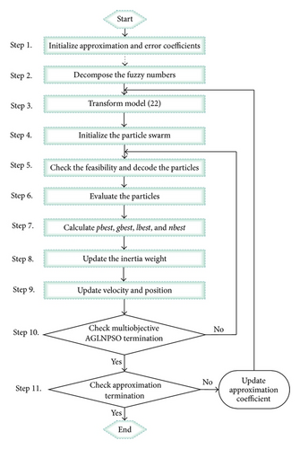
Step 1. Initialize approximation coefficient l = 1, which is used to generate cut sets for the fuzzy numbers in model (36) and the error coefficient ϵ.

Step 2. Decompose interval [0,1] into 2^l−1 equal sub-intervals with (2^l−1 + 1) nodes λ_i (i = 0, …, 2^l−1), which are arranged in the order .

Step 3. Transform model (34) into a series of models for model (36) with l.

Step 4. Initialize the parameters: swarm_size, iteration_max, the range of velocity and position for the variables, the personal best position acceleration constant, the global best position acceleration constant, the local best position acceleration constant, the near neighbor best acceleration constant, and the inertia weight_max. Then, initialize the velocities and positions of the particle-represented solutions.

Step 5. Check the feasibility and decode the particles.

Step 6. Solve the lower-level programming with the feasible solutions of the upper level to determine the optimal objective value. Calculate the two objectives on the upper level to evaluate every particle.

Step 7. Calculate the pbest, gbest, lbest, and nbest using the multiobjective method. Restore the Pareto optimal solutions (i.e., the (global) elite individuals), lower-level programming solutions, and objective values of upper level and lower level.

Step 8. Update the inertia weight for each iteration.

Step 9. Update the velocity and position of each particle.

Step 10. Check the multiobjective AGLNPSO termination. If the stopping criterion (i.e., iteration_max) is met, then end the multiobjective AGLNPSO procedure to obtain the optimal solution and go to Step 10; otherwise, go to Step 5.

Step 11. Check the approximation termination. If a stabilization of the Pareto optimal solution is achieved, then the Pareto optimal solution for the complete multiobjective bilevel programming model under fuzzy random environments is obtained, and it terminates. Otherwise, l = l + 1; go back to Step 3.

Here, the set convergence is proposed in this paper to describe the stabilization of the Pareto optimal solution, which is defined as ϖ and expressed as follows:

(37)

That is to say, if ϖ ≥ ϵ, the Pareto optimal solution set is stable and the approximation termination is achieved.

The details for the multiobjective AGLNPSO are described as follows and the notations used are shown.

s Particle index, s = 1, …, S
τ Iteration index, τ = 1, …, T
h Dimension index, h = 1, …, H
u_r Uniform random number in the interval [0,1]
w(τ) Inertia weight in the τth iteration
w^max Maximum inertia weight value
w^min Minimum inertia weight value
ω_sh(τ) Velocity of the sth particle at the hth dimension in the τth iteration
θ_sh(τ) Position of the sth particle at the hth dimension in the τth iteration
Position for temporary and noncritical link of the sth particle at the hth dimension in the τth iteration
ψ_sh Personal best position of the sth particle at the hth dimension
ψ_gh Global best position of the sth particle at the hth dimension
Local best position of the sth particle at the hth dimension
Near neighbor best position of the sth particle at the hth dimension
c_p Personal best position acceleration constant
c_g Global best position acceleration constant
c_l Local best position acceleration constant
c_n Near neighbor best position acceleration constant
ω^max Maximum velocity value
ω^min Minimum velocity value
θ^max Maximum position value
θ^min Minimum position value
Θ_s Vector position of the sth particle [θ_s1, θ_s2, …, θ_sH]
Ω_s Vector velocity of the sth particle [ω_s1, ω_s2, …, ω_sH]
R_s The sth set of solutions
c The current solution randomly selected one from the nondominated solutions
c^N New generated solution.

3.2. Solution Representation

In this paper, the particle-represented solution is A dimensions of retrofit rank u_a within [0,1, 2,3, 4,5] (i.e., a ∈ A) for all links in the LSCP transportation network.

3.3. Particle Swarm Initialization

Initialize S particles as a swarm; generate the sth particle with random position Θ_s in the range {0,1, 2,3, 4,5}. Randomly generate velocity for each particle in the range {−5, −4, −3, −2, −1,0, 1,2, 3,4, 5}. Set the iteration τ = 1. Set swarm_size S, iteration_max T, personal best position acceleration constant c_p, global best position acceleration constant c_g, local best position acceleration constant c_l, near neighbor best position acceleration constant c_n, inertia weight_max w^max, and inertia weight_min w^min.

3.4. Feasibility Checking and Decoding Method

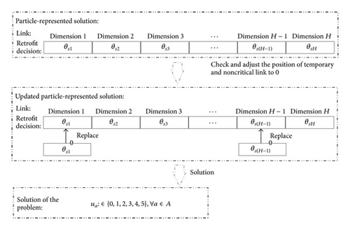
Since the links to be considered for retrofit are either permanent or critical, check and adjust the position of the temporary and noncritical links to 0. Then, the particle-represented solution can be directly decoded into a solution for the problem as shown in Figure 6.

3.5. Particle Evaluation

For s = 1, …, S, set Θ_s(τ) into the solution R_s that is u in the upper-level programming and put u into the lower-level programming to determine the optimal solution x and the optimal objective Q(x). Calculate another objective for the upper-level programming C(u).

3.6. Multiobjective Method

The multiobjective method is made up of the PAES procedure and the test procedure, and selection is introduced to calculate pbest, gbest, lbest, and nbest. This method uses a truncated archive to store the elite individuals (i.e., nondominated solutions), which is used to separate the objective function space into hypercubes, each of which has a score based on its density. Selection of the best is then based on a roulette wheel selection to select the best hypercube first and then uniformly choose a solution. Note that the initialized solution is regarded as the pbest and the nondominated solution of each particle at the 1th iteration. When the iteration updates, the updated solution and the nondominated solutions are used to calculate the pbest by the method. After the pbest has been confirmed at each iteration, the pbest nondominated solutions for all particles are considered with the gbest nondominated solutions (i.e., there is no gbest nondominated solution at initialization) to calculate the gbest by the method. Similar to the gbest, among all the pbest nondominated solutions from K neighbors of the sth particle and lbest nondominated solutions, set the lbest is also set using this method. For each particle on each dimension, set that maximizes (Z(Θ_s) − Z(Ψ_o))/(θ_sh − ψ_oh) to get nbest, o ∈ S∖s. Here, the maximization process uses the multiobjective method for the calculation of the gbest and lbest above. The details for the PAES procedure, test procedure, and selection procedure are outlined similarly for the pbest, gbest, lbest, and nbest next and in Procedures 1 and 2, where c is the current solution randomly selected from the nondominated solutions. Note that c is randomly selected from the pbest nondominated solutions to calculate the gbest at the 1th iteration.

Procedure 1: PAES.

generate a new solution c^N
if (c dominates c^N)
discard c^N
else if (c^N dominates c)
replace c with c^N and add c^N to the archive
else if (c^N is dominated by any member of the archive)
discard c^N
else if (c^N dominates any member of the archive)
replace it with c^N and add c^N to the archive and all other members
dominated by c^N are discarded
else
apply test procedure to c, c^N and the archive to determine which
becomes the new current solution and whether to add c^N to the archive
until a termination criterion has been reached, return to the beginning

Procedure 2: Test.

if the archive is not full
add c^N to the archive
if (c^N is in a less crowded region of the archive than c)
accept c^N as the new current solution
else
maintain c as the current solution
else if (c^N is in a less crowded region of the archive than any other member on the archive)
add c^N to the archive, and remove a member of the archive from the most crowded region
if (c^N is in a less crowded region of the archive than c)
accept c^N as the new current solution
else
maintain c as the current solution
else
don’t add c^N to the archive

Selection

Step 1. Divide 10 by the number of particles in each hypercube to get its score.

Step 2. Apply roulette wheel selection to hypercube according to their scores and select a hypercube.

Step 3. Uniformly choose a member of that hypercube.

Therefore, the gbest nondominated solutions at the Tth are the final solutions of the problem.

3.7. Inertia Weight Updating

Update the inertia weight for iteration τ using the following equations:

(38)

3.8. Velocity and Position Updating

Update the velocity and the position of each sth particle using the following equations:

(39)

4. A Case Study

In this section, computational experiments were carried out on a large-scale water conservancy and hydropower construction project. Through the illustrative example on the data set adopted from the case problem, the proposed approach is validated and the efficiency of the algorithm is tested.

4.1. Presentation of Case Problem

The XLD hydropower station LSCP is in XLD gorge section of the JS river located in LB county of SC province and YS county of YN province, an area which is earthquake prone. The Yingjiang, Wenchuan, and Panzhihua-Huili earthquakes all seriously affected the local area. Therefore, it is critical that the LSCP risks be controlled, especially in the transportation network. Therefore, the proposed approach is suitable for use on the transportation network at the XLD hydropower LSCP.

The transportation network in the project has an internal road network and an external road network. The internal road network is composed of more than 20 major trunk roads and these roads form a solid network located on the left and right banks. There is a temporary traffic bridge upstream and a permanent traffic bridge downstream. The external road network is composed of several secondary roads used for automobiles, which begins at the project dam and terminates at the PED railway station. In order to apply the proposed approach more conveniently, adjacent roads of the same type have been combined and the concrete shapes of the roads have been ignored. A simplified transportation network illustration is shown in Figure 7 which distinguishes the permanent and temporary, critical and noncritical nature of each road according to the practical location of the transportation network. The illustration has 24 nodes and 18 and 29 links. There are 12 commodities in total, which represent travel between different origin-destination pairs. The 16 nodes in these commodities have certain capacities (unit: number of vehicles (n)) and others have no capacity. Tables 1 and 2 give the detailed data.

Table 1. Travel of the commodities.

Commodity k	Travel of commodity
1′	#24 → #23 → #22 → #21 → #20
2′	#20 → #21 → #22 → #23 →#24
3′	#20 → #19 → #7→ #5 → #2
4′	#2 → #5 → #7 → #19 → #20
5′	#6 → #7 → #19 → #20
6′	#20 → #19 → #7 → #6
7′	#20 → #18 → #17 → #16 → #13
8′	#13 → #16 → #17 → #18 →#20
9′	#20 → #18 → #17 → #16 → #14
10′	#14 → #16 → #17 → #18 →#20
11′	#20 → #18 → #17 → #16 → #15
12′	#15 → #16 → #17 → #18 → #20

Table 2. Capacity of node.

Node b	#24	#23	#22	#21	#20	#19	#7	#5	#2	#6	#18	#17	#16	#13	#14	#15
Capacity ca_b (n)	51	51	51	51	149	49	49	22	22	25	49	49	49	16	18	15

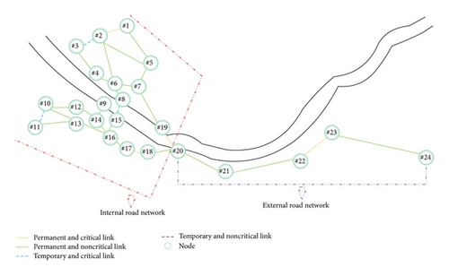
For each link in the transportation network, there is a free flow travel time (unit: hour (h)), a “practical capacity” for the link (unit: number of vehicles (n)), which is set to be 90% of the design capacity [1], and a fuzzy random seismic damage scenario . The corresponding data for this case problem are stated in Table 3. It should be noted that the probabilities assigned to the fuzzy numbers for the fuzzy random numbers in Table 3 were obtained through a statistical analysis of the historical data in the area.

Table 3. Free flow travel time

, practical capacity

, and fuzzy random seismic damage scenario

of each link.

Link a	Corresponding nodes b	Free flow travel time (h)	Practical capacity (n)
1	#1, #2	0.10	72

2	#2, #3	0.08	75

3 4 5 6 7 8 9 10 11	#1, #5 #2, #5 #2, #6 #3, #4 #4, #6 #6, #7 #5, #7 #6, #8 #7, #19	0.25	87

12	#19, #20	0.10	101

13	#10, #11	0.05	96

14 15 16 17 18 19 20 21 23 25	#1, #5 #12, #14 #14, #16 #9, #14 #11, #13 #13, #16 #10, #13 #15, #16 #16, #17 #18, #20	0.30	90

22	#8, #15	0.09	89

24	#17, #18	0.10	84

26 27 29	#20, #21 #21, #22 #23, #24	0.40	126

28	#22, #23	0.15	96

In the case problem, there are 2 outputs—the retrofit of permanent (i.e., i = 1) and temporary (i.e., i = 2) links. The activity process and activities for the retrofit are the same for both types of links. Activities (i.e., j = 1, …, 10) are as (1) breaking pavement, (2) digging grooves, (3) laying pipes, (4) backfilling grooves, (5) strengthening earth-rock, (6) evening roadbeds, (7) digging gutters, (8) building kerbstones, (9) constructing bases, (10) constructing pavements. Every activity corresponds to an activity cost center. According to [25], 5 environmental media can be determined in the retrofit work: (1) air and climate, (2) waste water, (3) waste, (4) soil and ground water, (5) noise and vibration. Environmental cost categories are recorded as in [25].

(1)
Waste and emission treatment: depreciation for related equipment; maintenance, operating materials and services; related personnel; fees, taxes, and charges; insurance for environmental liabilities.
(2)
Prevention and environmental management: external services for environmental management and personnel for general environmental management activities.
(3)
Material purchase value of nonproduct output: raw materials; auxiliary materials; operating materials; packaging; energy; and water.
(4)
Processing costs of nonproduct output: depreciation for machinery and labor hours.

Since categories 1, 3, and 4 are variable costs (i.e., v = 1,2, 3), category 2 is fixed costs (i.e., f = 1); they are recoded as (unit: ¥) , , and . Based on the descriptions above, the environmental costs of the retrofit are allocated as shown in Figure 8.

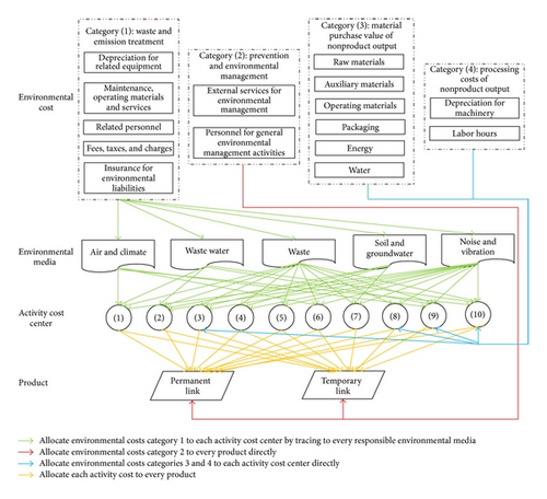
Based on the practice of the case problem and Figure 8, the percentage output for the fixed environmental costs 1 is . To calculate the final environmental costs for each output, the corresponding data for the activity cost centers j = 1, …, 10 is used as in Table 4. The percentage of j in the variable environmental cost categories is denoted as . am_j denotes the cost driver amount in j and [am_1j, am_2j] denotes the cost driver amount of outputs in j.

Table 4. Corresponding data of activity cost centers.

Activity cost center j				am_j	am_1j	am_2j
1	15.6%	0.0%	0.0%	426.30 m²	408.10 m²	18.20 m²
2	6.7%	0.0%	0.0%	9.74 m³	9.32 m³	0.42 m³
3	6.7%	25.0%	25.0%	60.90 m	58.30 m	2.60 m
4	6.7%	0.0%	0.0%	3.35 m³	3.21 m³	0.14 m³
5	5.4%	0.0%	0.0%	25.58 m³	24.49 m³	1.09 m³
6	15.6%	0.0%	0.0%	426.30 m²	408.10 m²	18.20 m²
7	6.7%	0.0%	0.0%	0.61 m³	0.58 m³	0.03 m³
8	5.4%	25.0%	25.0%	60.90 m	58.30 m	2.60 m
9	15.6%	25.0%	25.0%	426.30 m²	408.1 m²	18.20 m²
10	15.6%	25.0%	25.0%	426.30 m²	408.10 m²	18.20 m²

In addition, the corresponding cost data for the retrofit and reconstruction are shown in Table 5. The values for the other model parameters are as follows: δ = 0.2, η = 0.6, ρ = 1, α = 0.25, β = 2, and γ = 1.

Table 5. Cost data of retrofit and reconstruction.

Item	Cost (¥)
Increased variable retrofit costs for permanent link by basic rank (i.e., rank 1)	16732
Variable retrofit costs for temporary link by basic rank (i.e., rank 1)	30528
Increased fixed retrofit costs for permanent link	14525
Fixed retrofit costs for temporary link	28637
Increased variable reconstruction cost for permanent link by basic rank (i.e., rank 1)	107052
Variable reconstruction cost for temporary link by basic rank (i.e., rank 1)	98063
Increased fixed reconstruction cost for permanent link	69894
Fixed reconstruction cost for temporary link	50183

4.2. Case Solution

The developed algorithm was adopted using MATLAB 7.0 on an Inter Core 2, 2.00 GHz clock pulse with 2048 MB memory. The algorithmic parameters for the case problem were set as follows: error coefficient ϵ = 0.9, swarm_size S = 20, iteration_max T = 100, inertia weight_max w^max = 0.9, inertia weight_min w^min = 0.1, personal best position acceleration constant c_p = 0.5, global best position acceleration constant c_g = 0.5, local best position acceleration constant c_l = 0.2, and near neighbor best acceleration constant c_n = 0.1.

After 8 iterations of the approximation decomposition, the approximation termination was achieved within 36 minutes on an average of 10 runs, which is time acceptable. The optimal solutions are shown in Tables 6 and 7. For all the Pareto optimal solutions on the upper level, the corresponding solutions on the lower level are the same. Table 6 shows a Pareto optimal solution set with 45 solutions on the upper level, where only 10 of the set are enumerated for convenience of expression. The investor is able to choose their preferred plan from the set. If they feel that the retrofit costs including environmental costs C are more important, they would choose the minimum costs plan and vice versa. Since there are fuzzy numbers in model (36), it cannot state crisp optimal objective values in final decision results. However, they are easy to be transformed into equivalent crisp forms by many fuzzy theories and it will not effect the decision.

Table 6. Pareto optimal solution set on the upperlevel.

Solution u_a		1*	2*	3*	4*	5*	6*	7*	8*	9*	10*	……
Link a	1	3	3	3	3	4	4	2	1	3	3	……
	2	4	3	4	3	4	4	1	5	2	4	……
	3	2	4	2	3	2	1	2	1	5	2	……
	4	2	2	3	3	5	1	3	3	1	3	……
	5	4	3	3	1	4	4	1	5	3	4	……
	6	3	4	3	3	5	2	5	3	3	3	……
	7	4	3	3	3	3	5	1	1	2	3	……
	8	2	3	2	3	1	1	3	4	3	3	……
	9	3	4	3	2	5	1	2	4	4	3	……
	10	3	3	3	2	3	3	4	1	3	2	……
	11	2	2	2	2	3	3	2	1	1	2	……
	12	3	3	4	2	2	3	3	4	2	4	……
	13	3	3	3	1	5	3	4	4	2	3	……
	14	4	3	4	1	1	5	3	2	3	3	……
	15	2	2	1	1	2	1	2	1	3	2	……
	16	3	2	3	3	3	3	3	4	1	3	……
	17	3	2	3	2	2	4	3	2	2	3	……
	18	3	2	3	3	3	4	4	1	1	3	……
	19	3	3	2	5	1	2	5	1	3	2	……
	20	2	3	2	2	2	2	2	2	4	3	……
	21	2	4	2	5	1	1	4	3	5	4	……
	22	3	3	3	5	4	1	4	3	4	2	……
	23	2	3	2	5	2	1	2	2	3	2	……
	24	2	2	3	4	1	2	3	4	2	2	……
	25	3	2	3	2	3	3	1	5	2	3	……
	26	2	2	2	3	1	1	3	1	1	2	……
	27	4	3	4	1	3	4	3	3	2	3	……
	28	3	2	3	3	3	5	2	3	1	3	……
	29	4	4	4	5	4	5	2	5	3	4	……

Table 7. Optimal solutions on the lowerlevel.

Commodity k	1′	2′	3′	4′	5′	6′	7′	8′	9′	10′	11′	12′
Flow of commodity x_k (n/h)	25.50	25.50	12.00	12.00	12.50	12.50	8.00	8.00	9.00	9.00	7.50	7.50

4.3. Analytic Results of the Proposed Approach

(1) Worthiness of Modeling and Solutions. Fuzzy random programming approach explicitly considers the entire range of uncertain scenarios and thus is more conforming to reality for hedging better against uncertainty. Although it increases the complexity of modeling, the model is well transformed orienting computer implementation. In addition, the computing complexity of the model is not greater than that of the stochastic programming approach used in [1]. Therefore, the extra effort on modeling and solving fuzzy random bilevel programming is worthwhile.

The multiobjective method is introduced to determine the Pareto optimal solution set for the upper level and provides more effective and nondominated alternatives for the decision-maker. Compared with the weight-sum method for multiobjective in [19], the solutions in this paper have more reference value for the decision-maker and reflect the users’ preference requirements. Therefore, it is more worthwhile.

(2) Efficiency of Algorithm. This paper compares GA, an usually used metaheuristics algorithm, and the developed algorithm in this study. The merit of GA is its strong evolutionary process to find an optimal solution by the operation of crossover, mutation, and selection. However, the randomly generated initial generation at the algorithms’ beginning affects the solution quality because of the bad gene inherited from the parent generation. Moreover, the searching capability is reduced as GA does not rely on gradient or derivative information. In the developed algorithm, the particle-represented solutions closely connect the particles of PSO and the solutions to the problem. The hybrid particle-updating mechanism successfully enhances the searching capability. The developed algorithm is a useful tool for the solution to the problem. In contrast to the previous papers, such as [19, 21], both the bilevel and multiobjective environments are considered in this paper.

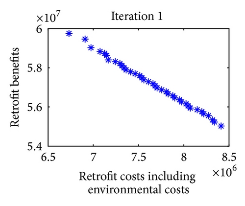
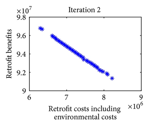
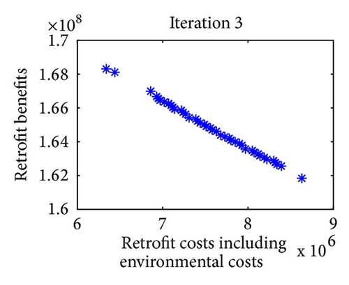
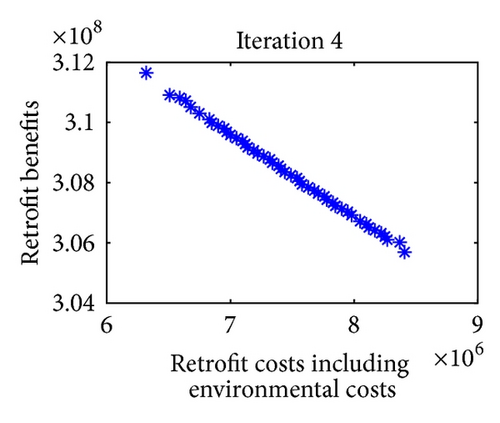
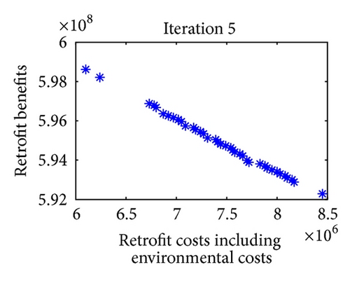
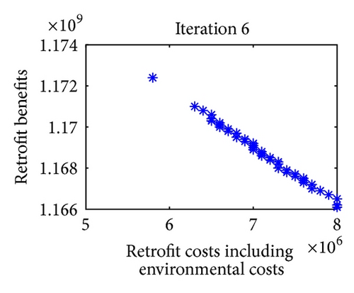
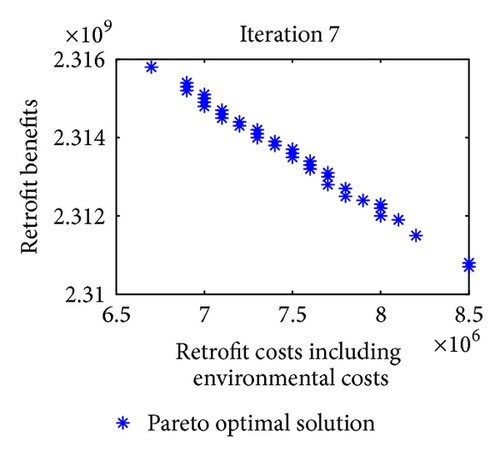
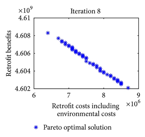
For multiobjective optimization, the definition of quality is substantially more complex than for single-objective optimization problems. Figure 9 shows the iterative results of Pareto optimal solutions in 8 iterations. Note that in each iteration of approximation decomposition, these fuzzy numbers in model (36) are decomposed into crisp forms. Therefore, the objective values can be evaluated. For further expression of the efficiency of the convergence, three metrics of performance are studied. Table 8 shows the metrics of performance for Pareto optimal sets proposed in [51] and the set convergence of Pareto optimal sets in 8 iterations after 10 runs.

Table 8. Metrics of performance and set convergence for Pareto optimal sets.

Iteration	The average distance	The distribution	The extent	The set convergence
1	0.0812	0.5623	5.0088	—
2	0.0630	0.4615	5.7706	Iteration 1–2: 0.5610
3	0.1364	0.8600	6.8594	Iteration 2–3: 0.6765
4	0.1223	0.5250	6.3147	Iteration 3–4: 0.7632
5	0.1502	0.6820	6.7538	Iteration 4–5: 0.8750
6	0.2835	0.9600	6.6417	Iteration 5–6: 0.8571
7	0.0973	0.5289	5.4451	Iteration 6–7: 0.5712
8	0.1300	0.8635	6.6424	Iteration 7–8: 0.9143

(3) Efficiency of Algorithm Parameters. Since the search space for the problem is so large and the computing process is time-consuming, it is necessary to choose reasonable algorithm parameters. Table 9 shows the comparison results of different swarm_size (i.e., S) and iteration_max (i.e., T) on average computing time and iterations after 10 runs. Looking into Table 9, when S = 10, the program could not obtain results in more than 3600 s and more than 10 iterations with both T = 100 and T = 200. This is the same when S = 50 with the lower iterations. When S = 20 and T = 200, the process is more time-consuming than the current algorithm parameters. Therefore, the current ones are considered suitable.

Table 9. Comparison of different algorithm parameters.

	S = 10		S = 20		S = 50
	T = 100	T = 200	T = 100	T = 200	T = 100	T = 200
Computing time (s)	≥3600	≥3600	2160	3480	≥3600	≥3600
Iterations	≥16	≥12	8	6	≥4	≥3

5. Conclusions

This paper studies retrofit decision for transportation network of LSCP to hedge against seismic risk. On the consideration of the emerged challenges in the problem, using distinctions of various link types, bilevel decision, environmental costs, and fuzzy random seismic damage scenario, a fuzzy random multiobjective bilevel programming model is set up. A transforming approach is in use to obtain equivalent fuzzy bilevel programming model. Then, decomposition is utilized to these fuzzy variables by decomposition theorem of fuzzy number. An approximation decomposition-based multiobjective AGLNPSO is developed to solve the problem. A case study is presented as an illustrative example of this problem. The results validate the worthiness of modeling and solutions and test the efficiency of the algorithm and parameters.

The contributions of this paper to literature are as the follows. (1) This study adopts the work of [1] to the filed of LSCP. Bilevel decision involves, with the investor and the administer, distinctions of various link types, and retrofit decision specified into several ranks according to the seismic damage scenario provides more reasonable and practical description of the problem. (2) Although there are many works on environmental cost, such as [25, 26], few papers consider it in transportation network in LSCP. Thus it enhances the focus points of management aims of the problem. (3) This paper uses fuzzy random seismic damage scenario to describe the hybrid uncertain situation. To the best of our knowledge, it has never been done before. (4) The approximation decomposition-based multiobjective AGLNPSO is developed as one of the useful tools to solve this problem. In contrast to the previous papers, such as [19, 21], both the bilevel and multiobjective environments are considered in this paper.

There are three areas suggested for future research. First, more cost categories need to be investigated and the detailed relationships between the retrofit decision and the costs should be outlined to ensure the model is as practical as possible. Secondly, to determine better, more effective solutions with lower memory and computing time requirements, alternative approaches and algorithms (e.g., other exact approaches, (meta)heuristics, evolutionary algorithms, etc.) could be used to make comparisons. Finally, consideration of other behavior assumptions, such as the travelers learning or user equilibrium, may change the structure of the problem. Each of these areas is very important and equally worthy of our concern.

Conflict of Interests

The authors declare no conflict of interests.

Acknowledgments

This research was supported by the Key Program of NSFC (Grant no. 70831005), “985” Program of Sichuan University “Innovative Research Base for Economic Development and Management,” and the Research Foundation of Ministry of Education for the Doctoral Program of Higher Education of China (Grant no. 20130181110063).

References

1 Liu C., Fan Y., and Ordóñez F., A two-stage stochastic programming model for transportation network protection, Computers and Operations Research. (2009) 36, no. 5, 1582–1590, 2-s2.0-55749085781, https://doi.org/10.1016/j.cor.2008.03.001, ZBL1179.90246.
10.1016/j.cor.2008.03.001
Web of Science® Google Scholar
2 Werner S. D., Taylor C. E., Moore J. E., and Walton J. S., Seismic Retrofitting Manuals for Highway Systems, Volume I, Seismic Risk Analysis of Highway Systems, and Technical Report for Volume I, 1999, Multidisciplinary Center for Earthquake Engineering Research, Buffalo, NY, USA.
Google Scholar
3 Sohn J., Kim T. J., Hewings G. J. D., Lee J. S., and Jang S.-G., Retrofit priority of transport network links under an earthquake, Journal of Urban Planning and Development. (2003) 129, no. 4, 195–210, 2-s2.0-0347029827, https://doi.org/10.1061/(ASCE)0733-9488(2003)129:4(195).
10.1061/(ASCE)0733-9488(2003)129:4(195)
Web of Science® Google Scholar
4 Priestley M. J. N., Seible F., and Calvi G. F., Seismic Design and Retrofit of Bridges, 1996, John Wiley & Sons, New York, NY, USA.
10.1002/9780470172858
Google Scholar
5 Shinozuka M., Murachi Y., Dong X., Zhou Y., and Orlikowski M. J., Effect of seismic retrofit of bridges on transportation networks, Earthquake Engineering and Engineering Vibration. (2003) 2, no. 2, 169–179, 2-s2.0-4544220005.
10.1007/s11803-003-0001-0
Google Scholar
6 Zhou Y., Banerjee S., and Shinozuka M., Socio-economic effect of seismic retrofit of bridges for highway transportation networks: a pilot study, Structure and Infrastructure Engineering. (2010) 6, no. 1-2, 145–157, 2-s2.0-77951628451, https://doi.org/10.1080/15732470802663862.
10.1080/15732470802663862
Web of Science® Google Scholar
7 Kwakernaak H., Fuzzy random variables-I. Definitions and theorems, Information Sciences. (1978) 15, no. 1, 1–29, 2-s2.0-6344232554, https://doi.org/10.1016/0020-0255(78)90019-1, ZBL0438.60004.
10.1016/0020-0255(78)90019-1
Web of Science® Google Scholar
8 Zhao R., Tang W., and Wang C., Fuzzy random renewal process and renewal reward process, Fuzzy Optimization and Decision Making. (2007) 6, no. 3, 279–295, 2-s2.0-34848917333, https://doi.org/10.1007/s10700-007-9012-z, ZBL1138.60057.
10.1007/s10700-007-9012-z
CAS Web of Science® Google Scholar
9 Fei W., A generalization of bihari′s inequality and fuzzy random differential equations with non-Lipschitz coefficients, International Journal of Uncertainty, Fuzziness and Knowlege-Based Systems. (2007) 15, no. 4, 425–439, 2-s2.0-34548255362, https://doi.org/10.1142/S0218488507004777, ZBL1149.26038.
10.1142/S0218488507004777
Web of Science® Google Scholar
10 Shapiro A. F., Fuzzy random variables, Insurance. (2009) 44, no. 2, 307–314, 2-s2.0-63749130587, https://doi.org/10.1016/j.insmatheco.2008.05.008, ZBL1166.91018.
10.1016/j.insmatheco.2008.05.008
Google Scholar
11 Liu Y. K. and Gao J., The independence of fuzzy variables with applications to fuzzy random optimization, International Journal of Uncertainty, Fuzziness and Knowlege-Based Systems. (2007) 15, no. supplement 2, 1–20, 2-s2.0-34249009221.
10.1142/S021848850700456X
CAS Web of Science® Google Scholar
12 Xu J. P. and Liu Y. G., Multi-objective decision making model under fuzzy random environment and its application to inventory problems, Information Sciences. (2008) 178, no. 14, 2899–2914, 2-s2.0-43849106075, https://doi.org/10.1016/j.ins.2008.03.003, ZBL1146.90067.
10.1016/j.ins.2008.03.003
Web of Science® Google Scholar
13 Xu J. and Zhang Z., A fuzzy random resource-constrained scheduling model with multiple projects and its application to a working procedure in a large-scale water conservancy and hydropower construction project, Journal of Scheduling. (2012) 15, no. 2, 253–272, 2-s2.0-77950937767, https://doi.org/10.1007/s10951-010-0173-1.
10.1007/s10951-010-0173-1
Web of Science® Google Scholar
14 Puri M. L. and Ralescu D. A., Fuzzy random variables, Journal of Mathematical Analysis and Applications. (1986) 114, no. 2, 409–422, 2-s2.0-0022674414, https://doi.org/10.1016/0022-247X(86)90093-4, ZBL0605.60038.
10.1016/0022-247X(86)90093-4
Web of Science® Google Scholar
15 Klement E. P., Puri M. L., and Ralescu D. A., Limit theorems for fuzzy random variables, Proceedings of The Royal Society of London A. (1986) 407, no. 1832, 171–182, MR861082, https://doi.org/10.1098/rspa.1986.0091, ZBL0605.60038.
10.1098/rspa.1986.0091
Web of Science® Google Scholar
16 Gil M. Á., López-Díaz M., and Ralescu D. A., Overview on the development of fuzzy random variables, Fuzzy Sets and Systems. (2006) 157, no. 19, 2546–2557, 2-s2.0-33748062355, https://doi.org/10.1016/j.fss.2006.05.002, ZBL1108.60006.
10.1016/j.fss.2006.05.002
Web of Science® Google Scholar
17 Kruse R. and Meyer K. D., Statistics with Vague Data, 1987, D. Reidel Publishing, Dordrecht, The Netherlands, https://doi.org/10.1007/978-94-009-3943-1, MR913303.
10.1007/978-94-009-3943-1
Google Scholar
18 Xu J., Yan F., and Li S., Vehicle routing optimization with soft time windows in a fuzzy random environment, Transportation Research E. (2011) 47, no. 6, 1075–1091, 2-s2.0-79960968882, https://doi.org/10.1016/j.tre.2011.04.002.
10.1016/j.tre.2011.04.002
Google Scholar
19 Zhang G., Lu J., and Dillon T., Decentralized multi-objective bilevel decision making with fuzzy demands, Knowledge-Based Systems. (2007) 20, no. 5, 495–507, 2-s2.0-34248145961, https://doi.org/10.1016/j.knosys.2007.01.003.
10.1016/j.knosys.2007.01.003
Web of Science® Google Scholar
20 Knowles J. D. and Corne D. W., Approximating the nondominated front using the pareto archived evolution strategy, Evolutionary Computation. (2000) 8, no. 2, 149–172, 2-s2.0-0034199912, https://doi.org/10.1162/106365600568167.
10.1162/106365600568167
CAS PubMed Web of Science® Google Scholar
21 Ai T. J., Particle Swarm Optimization for Generalized Vehicle Routing Problem [Doctoral Dissertation], 2008, Asian Institute of Technology, Thailand.
Google Scholar
22 Ueno G., Yasuda K., and Iwasaki N., Robust adaptive particle swarm optimization, Proceedings of the IEEE International Conference on Systems, Man, Cybernetics, October 2005, 3915–3920, 2-s2.0-27944502521.
Google Scholar
23 Ai T. J. and Kachitvichyanukul V., A particle swarm optimization for the vehicle routing problem with simultaneous pickup and delivery, Computers and Operations Research. (2009) 36, no. 5, 1693–1702, 2-s2.0-56049086164, https://doi.org/10.1016/j.cor.2008.04.003, ZBL1179.90068.
10.1016/j.cor.2008.04.003
Web of Science® Google Scholar
24 Coello C. A. C. and Lechunga M. S., MOPSO: a proposal for multiple objective particle swarm optimization, Proceedings of the IEEE Word Congress on Computational Intelligence, 2002, https://doi.org/10.1016/j.cor.2008.04.003.
10.1016/j.cor.2008.04.003
Google Scholar
25 Jasch C., The use of environmental management accounting (EMA) for identifying environmental costs, Journal of Cleaner Production. (2003) 11, no. 6, 667–676, 2-s2.0-0037411990, https://doi.org/10.1016/S0959-6526(02)00107-5.
10.1016/S0959-6526(02)00107-5
Web of Science® Google Scholar
26 Xiao X., Theory of Environment Cost, 2002, China Financial & Economic Publishing House, Beijing, China.
Google Scholar
27 Cooper R., The rise of activity-based costing part one: what is an activity-based cost system?, Journal of Cost Management. (1988) 2, 45–54.
Google Scholar
28 Cooper R., The rise of activity-based costing part two: when do I need an activity-based cost system?, Journal of Cost Management. (1988) 2, 41–48.
Google Scholar
29 Cooper R., The rise of activity-based costing part three: how many cost drivers do you need, and how do you select them?, Journal of Cost Management. (1989) 2, 34–46.
Google Scholar
30 Cooper R., The rise of activity-based costing part four: what do activity-based cost systems look like?, Journal of Cost Management. (1989) 3, 34–46.
Google Scholar
31 Kaplan R. S., Measuring manufacturing performance: a new challenge for managerial accounting research, The Accounting Review. (1983) 58, 686–705.
Web of Science® Google Scholar
32 Kaplan R. S., Yesterday’s accounting undermines production, Harvard Business Review. (1984) 95–101.
Web of Science® Google Scholar
33 Zadeh L. A., Fuzzy sets, Information and Control. (1965) 8, no. 3, 338–353, 2-s2.0-34248666540, https://doi.org/10.1016/S0019-9958(65)90241-X, ZBL0139.24606.
10.1016/S0019-9958(65)90241-X
CAS Web of Science® Google Scholar
34 Krätschmer V., A unified approach to fuzzy random variables, Fuzzy Sets and Systems. (2001) 123, no. 1, 1–9, 2-s2.0-0035480420, https://doi.org/10.1016/S0165-0114(00)00038-5, ZBL1004.60003.
10.1016/S0165‐0114(00)00038‐5
Web of Science® Google Scholar
35 Li J., Xu J., and Gen M., A class of multiobjective linear programming model with fuzzy random coefficients, Mathematical and Computer Modelling. (2006) 44, no. 11-12, 1097–1113, 2-s2.0-33746868300, https://doi.org/10.1016/j.mcm.2006.03.013, ZBL1165.90701.
10.1016/j.mcm.2006.03.013
Google Scholar
36 Liu Y.-K. and Liu B., Fuzzy random variables: a scalar expected value operator, Fuzzy Optimization and Decision Making. (2003) 2, no. 2, 143–160, 2-s2.0-0042003111, https://doi.org/10.1023/A:1023447217758.
10.1023/A:1023447217758
CAS Web of Science® Google Scholar
37 López-Díaz M. and Gil M. A., The λ-average value and the fuzzy expectation of a fuzzy random variable, Fuzzy Sets and Systems. (1998) 99, no. 3, 347–352, 2-s2.0-0040987826, https://doi.org/10.1016/S0165-0114(97)00031-6, ZBL0941.60030.
10.1016/S0165-0114(97)00031-6
Web of Science® Google Scholar
38 Özdamar L. and Demir O., A hierarchical clustering and routing procedure for large scale disaster relief logistics planning, Transportation Research E. (2012) 48, no. 3, 591–602, 2-s2.0-84856353289, https://doi.org/10.1016/j.tre.2011.11.003.
10.1016/j.tre.2011.11.003
Google Scholar
39 Dubois D. and Prade H., Possibility Theory: An Approach to Computerized Processing of Uncertainty, 1988, Plenum Press, New York, NY, USA, https://doi.org/10.1007/978-1-4684-5287-7, MR1104217.
10.1007/978-1-4684-5287-7
Google Scholar
40 Nahmias S., Fuzzy variables, Fuzzy Sets and Systems. (1978) 1, no. 2, 97–110, 2-s2.0-0002194031, https://doi.org/10.1016/0165-0114(78)90011-8, ZBL0383.03038.
10.1016/0165-0114(78)90011-8
Google Scholar
41 Zhang G., Lu J., and Gao Y., An algorithm for fuzzy multi-objective multi-follower partial cooperative bilevel programming, Journal of Intelligent and Fuzzy Systems. (2008) 19, no. 4-5, 303–319, 2-s2.0-55349128188, ZBL1211.90221.
Web of Science® Google Scholar
42 Bard J. F., Some properties of the bilevel programming problem, Journal of Optimization Theory and Applications. (1991) 68, no. 2, 371–378, 2-s2.0-0026114683, https://doi.org/10.1007/BF00941574, ZBL0696.90086.
10.1007/BF00941574
Web of Science® Google Scholar
43 Yao L. and Xu J., A class of expected value bilevel programming problems with random coefficients based on rough approximation and its application to a production-inventory system, Abstract and Applied Analysis. (2013) 2013, 12, 312527, MR3064333, ZBL06209254, https://doi.org/10.1155/2013/312527.
10.1155/2013/312527
Google Scholar
44 Bard J. F. and Falk J. E., An explicit solution to the multi-level programming problem, Computers and Operations Research. (1982) 9, no. 1, 77–100, 2-s2.0-0019937742, https://doi.org/10.1016/0305-0548(82)90007-7.
10.1016/0305-0548(82)90007-7
Web of Science® Google Scholar
45 Fortuny-Amat J. and McCarl B., A representation and economic interpretation of a two-level programming problem, Journal of the Operational Research Society. (1981) 32, no. 9, 783–792, 2-s2.0-0019608634, ZBL0459.90067.
10.1057/jors.1981.156
Web of Science® Google Scholar
46 Vicente L., Savard G., and Júdice J., Descent approaches for quadratic bilevel programming, Journal of Optimization Theory and Applications. (1994) 81, no. 2, 379–399, 2-s2.0-0028425698, https://doi.org/10.1007/BF02191670, ZBL0819.90076.
10.1007/BF02191670
Web of Science® Google Scholar
47 Case L. M., An l1 Penalty Function Approach to the Nonlinear Bilevel Programming Problem [Ph.D. thesis], 1999, University of Waterloo, Ottawa, Canada.
Google Scholar
48 Lucio B., Massimiliano C., and Stefano G., A bilevel flow model for hazmat transportation network design, Transportation Research C. (2009) 17, no. 2, 175–196, 2-s2.0-61349162912, https://doi.org/10.1016/j.trc.2008.10.001.
10.1016/j.trc.2008.10.001
Web of Science® Google Scholar
49 Gao Y., Zhang G., Lu J., and Wee H.-M., Particle swarm optimization for bi-level pricing problems in supply chains, Journal of Global Optimization. (2011) 51, no. 2, 245–254, 2-s2.0-80053332041, https://doi.org/10.1007/s10898-010-9595-8, ZBL1230.90179.
10.1007/s10898-010-9595-8
Web of Science® Google Scholar
50 Cagnina L., Esquivel S., and Coello C. A. C., A particle swarm optimizer for multi-objective optimization, Journal of Computer Science and Technology. (2005) 5, no. 4, 204–210.
Google Scholar
51 Zitzler E., Deb K., and Thiele L., Comparison of multiobjective evolutionary algorithms: empirical results, Evolutionary Computation. (2000) 8, no. 2, 173–195, 2-s2.0-0034199979, https://doi.org/10.1162/106365600568202.
10.1162/106365600568202
CAS PubMed Web of Science® Google Scholar

Citing Literature

All articles

Retrofitting Transportation Network Using a Fuzzy Random Multiobjective Bilevel Model to Hedge against Seismic Risk

Abstract

1. Introduction

2. Modeling

2.1. LSCP Transportation Network

2.2. Bilevel Decision Framework

2.3. Environmental Costs

2.4. Fuzzy Random Seismic Damage Scenario

2.5. Model Formulation

2.5.1. Upper-Level Programming

2.5.2. Lower-Level Programming

2.5.3. Fuzzy Random Multiobjective Bilevel Programming Model

2.6. Transformation Approach for Fuzzy Random Variables

2.7. Approximation Decomposition of Fuzzy Variables

3. An Approximation Decomposition-Based Multiobjective AGLNPSO

3.1. Overall Procedure for the Proposed Algorithm

3.2. Solution Representation

3.3. Particle Swarm Initialization

3.4. Feasibility Checking and Decoding Method

3.5. Particle Evaluation

3.6. Multiobjective Method

3.7. Inertia Weight Updating

3.8. Velocity and Position Updating

4. A Case Study

4.1. Presentation of Case Problem

4.2. Case Solution

4.3. Analytic Results of the Proposed Approach

5. Conclusions

Conflict of Interests

Acknowledgments

References

Citing Literature

Figures

References

Information

About Wiley Online Library

Help & Support

Opportunities

Connect with Wiley

Retrofitting Transportation Network Using a Fuzzy Random Multiobjective Bilevel Model to Hedge against Seismic Risk

Abstract

1. Introduction

2. Modeling

2.1. LSCP Transportation Network

2.2. Bilevel Decision Framework

2.3. Environmental Costs

2.4. Fuzzy Random Seismic Damage Scenario

2.5. Model Formulation

2.5.1. Upper-Level Programming

2.5.2. Lower-Level Programming

2.5.3. Fuzzy Random Multiobjective Bilevel Programming Model

2.6. Transformation Approach for Fuzzy Random Variables

2.7. Approximation Decomposition of Fuzzy Variables

3. An Approximation Decomposition-Based Multiobjective AGLNPSO

3.1. Overall Procedure for the Proposed Algorithm

3.2. Solution Representation

3.3. Particle Swarm Initialization

3.4. Feasibility Checking and Decoding Method

3.5. Particle Evaluation

3.6. Multiobjective Method

3.7. Inertia Weight Updating

3.8. Velocity and Position Updating

4. A Case Study

4.1. Presentation of Case Problem

4.2. Case Solution

4.3. Analytic Results of the Proposed Approach

5. Conclusions

Conflict of Interests

Acknowledgments

References

Citing Literature

Figures

References

Related

Information