RESEARCH ARTICLE

Open Access

An intelligent algorithm to fast and accurately detect chaotic correlation dimension

Mengyan Shen

orcid.org/0009-0002-5562-0015

Research Center on Flood and Drought Disaster Reduction of the Ministry of Water Resources, China Institute of Water Resources and Hydropower Research, Beijing, China

Key Laboratory of Water Safety for Beijing-Tianjin-Hebei Region of Ministry of Water Resources, Beijing, China

Search for more papers by this author

Miaomiao Ma,

Corresponding Author

Miaomiao Ma

[email protected]

Research Center on Flood and Drought Disaster Reduction of the Ministry of Water Resources, China Institute of Water Resources and Hydropower Research, Beijing, China

Key Laboratory of Water Safety for Beijing-Tianjin-Hebei Region of Ministry of Water Resources, Beijing, China

Correspondence Miaomiao Ma, Research Center on Flood and Drought Disaster Reduction of the Ministry of Water Resources, China Institute of Water Resources and Hydropower Research, Beijing 100038, China.

Email: [email protected]

Search for more papers by this author

Zhicheng Su,

Zhicheng Su

Research Center on Flood and Drought Disaster Reduction of the Ministry of Water Resources, China Institute of Water Resources and Hydropower Research, Beijing, China

Key Laboratory of Water Safety for Beijing-Tianjin-Hebei Region of Ministry of Water Resources, Beijing, China

Search for more papers by this author

Xuejun Zhang,

Xuejun Zhang

Research Center on Flood and Drought Disaster Reduction of the Ministry of Water Resources, China Institute of Water Resources and Hydropower Research, Beijing, China

Key Laboratory of Water Safety for Beijing-Tianjin-Hebei Region of Ministry of Water Resources, Beijing, China

Search for more papers by this author

Mengyan Shen,

Mengyan Shen

orcid.org/0009-0002-5562-0015

Research Center on Flood and Drought Disaster Reduction of the Ministry of Water Resources, China Institute of Water Resources and Hydropower Research, Beijing, China

Key Laboratory of Water Safety for Beijing-Tianjin-Hebei Region of Ministry of Water Resources, Beijing, China

Search for more papers by this author

Miaomiao Ma,

Corresponding Author

Miaomiao Ma

[email protected]

Research Center on Flood and Drought Disaster Reduction of the Ministry of Water Resources, China Institute of Water Resources and Hydropower Research, Beijing, China

Key Laboratory of Water Safety for Beijing-Tianjin-Hebei Region of Ministry of Water Resources, Beijing, China

Email: [email protected]

Search for more papers by this author

Zhicheng Su,

Zhicheng Su

Research Center on Flood and Drought Disaster Reduction of the Ministry of Water Resources, China Institute of Water Resources and Hydropower Research, Beijing, China

Key Laboratory of Water Safety for Beijing-Tianjin-Hebei Region of Ministry of Water Resources, Beijing, China

Search for more papers by this author

Xuejun Zhang,

Xuejun Zhang

Research Center on Flood and Drought Disaster Reduction of the Ministry of Water Resources, China Institute of Water Resources and Hydropower Research, Beijing, China

Key Laboratory of Water Safety for Beijing-Tianjin-Hebei Region of Ministry of Water Resources, Beijing, China

Search for more papers by this author

First published: 08 May 2025

https://doi.org/10.1002/rvr2.70008

Share a link

Email
Wechat
Bluesky

Abstract

Detecting the complexity of natural systems, such as hydrological systems, can help improve our understanding of complex interactions and feedback between variables in these systems. The correlation dimension method, as one of the most useful methods, has been applied in many studies to investigate the chaos and detect the intrinsic dimensions of underlying dynamic systems. However, this method often relies on manual inspection due to uncertainties from identifying the scaling region, making the correlation dimension value calculation troublesome and subjective. Therefore, it is necessary to propose a fast and intelligent algorithm to solve the above problem. This study implies the distinct windows tracking technique and fuzzy C-means clustering algorithm to accurately identify the scaling range and estimate the correlation dimension values. The proposed method is verified using the classic Lorenz chaotic system and 10 streamflow series in the Daling River basin of Liaoning Province, China. The results reveal that the proposed method is an intelligent and robust method for rapidly and accurately calculating the correlation dimension values, and the average operation efficiency of the proposed algorithm is 30 times faster than that of the original Grassberger-Procaccia algorithm.

1 INTRODUCTION

Complexity has become one of the most important measurements in nonlinear time series analysis in that it not only offers another description for nonlinear characteristics (e.g., chaoticity, fractality, irregularity, and long-range memorability) but also determines the features of inner factors (e.g., central trend, and cyclical, seasonal and mutable patterns) and their interrelationship (Tang et al., 2015). Thus, during the past few decades, numerous attempts have been made to define, qualify, and quantify complexity and also to apply complexity-based theories for studying natural and physical systems (Benmebarek & Chettih, 2023; Huang et al., 2020; Ogunjo et al., 2024; Shen et al., 2020; Sivakumar, 2017; Wang et al., 2019). Amongst them, the correlation dimension is an important indicator reflecting the system's complexity. As correlation dimension (CD) method can represent the essential features of a system using time series of only a single variable of the entire multi-variable system through a “pseudo” phase-space (or state-space) reconstruction, it has attracted considerable interest of scientists in atmospheric and hydrologic sciences (Di et al., 2023; Shu et al., 2023; Sivakumar, 2004a). The obtained CD value is extremely sensitive to slight changes in the complexity of the underlying deterministic structure (Decoster & Mitchell, 1991). The higher the CD value, the more complex the underlying system dynamics appear to be.

Grassberger-Procaccia algorithm (hereinafter denoted as the “G-P algorithm”), proposed by Grassberger and Procaccia (1983a, b), is used for calculating the CD values. However, this algorithm provides few criteria for the identification of scaling region. The term “scaling region” refers to the straight line portion of the curves in the $\log C (r)$ versus $\log r$ plot; however, due to data noise, the straight line corresponding to the scaling region is not a strict straight line, but a linear region of discrete points with gentle fluctuations, making the scaling region difficult to identify (Mcmahon et al., 2017). By now, “visual inspection” is a widely adopted method to determine the scaling region, yet it is quite difficult and troublesome for the users to identify the scaling region, thereby leading to inaccurate estimated CD values (Camastra et al., 2018). In light of this, many scholars have attempted to seek a systematic, objective, and fast method for identifying the scaling region. Based on different features, these studies can be divided into two main categories. First, some studies proposed the methods to fast identify the scaling region, but these methods lack not only theoretical basis but also certain objectivity. For example, Yokoya and Yamatomo (1989), Maragos & Fan-Kon Sun, 1993; Kim et al. (1999), Harikrishnan et al. (2006), and Jothiprakash and Fathima (2013) tried to obtain the upper limit of the scaling region using empirical equations; Wang et al. (1993) proposed a three-fold method, and Bolea et al. (2014) proposed a S-curve fitting method to identify the scaling region based on special curve models; Judd (1994) proposed Judd algorithm to calculate the CD values of special fractal systems; Dang and Huang (2004) proposed a method involving grouped recursive computer-recognition based on two so-called appraisal indices: confidence level and correlation. Second, other studies proposed methods to objectively identify the scaling region, but they are time-consuming and easy to fall into a certain value, or cause a bloated calculation, resulting in slow calculation for big data. For example, Wu (2002) proposed an adaptive method based on standard deviation to determine the scaling region; Jia et al. (2012), Du et al. (2013), and Wu et al. (2014) determined the scaling region based on piecewise fitting method; Yang et al. (2008) applied K-means clustering algorithm to identify the scaling region, and used classic chaotic attractors for verification; Ji et al. (2011) proposed a novel method based on the K-means algorithm and the point-slope-error algorithm to improve the calculational accuracy of the correlation dimension; Di et al. (2018) proposed an improved G-P algorithm, integrating the normal-based K-means clustering technique and random sample consensus algorithm, to calculate the correlation dimension. Chen et al. (2019) introduced a novel two-stage method using the K-means algorithm, which identifies the initial scaling region in the first stage, and refines this region to achieve greater accuracy in the second stage. Zhou et al. (2022) proposed a method using machine learning known as “density peak” based clustering algorithm to identify the scaling region. To sum up, these methods either lack certain objectivity or are time-consuming for big data, among other problems. In addition, these methods are not necessarily effective in many actual time series, such as streamflow, rainfall, groundwater, and temperature, even if they are useful in experimental data produced by ideal attractors. In this context, this paper tries to fill this gap and provides a method that can identify the scaling range rapidly and robustly.

The primary goals of this study are twofold: First, a new algorithm is proposed to improve the G-P algorithm, which integrates the distinct windows tracking technique and fuzzy C-means clustering algorithm. The classical Lorenz chaotic system is adopted to test the effectiveness of the proposed algorithm for estimating the CD values. Afterwards, the streamflow series in the Daling River basin is used for further verification. The rest of this paper is organized as follows: Section 2 describes the methods, including G-P algorithm and fuzzy C-means clustering algorithm, and data used in this paper. Section 3 presents the main findings of this paper. Finally, Sections 4 and 5 presents the discussion and conclusion.

2 METHODS AND DATA

In this study, we used the CD method to detect the intrinsic dimensionalities and dominant processes of the underlying dynamic system, which can help guide prediction model selection. To address the limitation of the original G-P algorithm for identifying the scaling region, the distinct windows tracking technique and the fuzzy C-means clustering algorithm were introduced to accurately and rapidly detect the CD values. First, the distinct window tracking technique was employed to divide the curve of

\log C (r)

versus

\log r

into 50 segments, and the slope of every segment was obtained by the least square method. Then, the fuzzy C-means clustering algorithm was used to cluster these slopes, and the appropriate cluster was selected to calculate mean slope, that is, the correlation exponent. The mean value of the saturation range of the correlation exponent versus the embedding dimension was the CD value. To make the CD value more reliable, this saturation range should be visible for at least three different time lags, which was verified by our extensive experiments. The three major calculation steps are as follows:

(1)
Reconstructing the phase space using the time delay embedding method to represent the underlying system dynamics.
(2)
Identifying the scaling region based on the distinct windows tracking technique and fuzzy C-means clustering algorithm for calculating the correlation exponent.
(3)
Plotting correlation exponent v versus embedding dimension m for different values of time lags, and then estimating the CD value as the mean value of the saturation range in the correlation exponent versus embedding dimension plot.

2.1 Correlation dimension method

The correlation dimension method can be used as a nonlinear time series analysis method based on the theory of dynamic systems. It has the following three advantages: First, as one of the nonlinear time series analysis methods, it can detect nonlinear characteristics of the time series. Second, it can detect the intrinsic dimensionalities and dominant processes of the underlying dynamic system, which are not subject to change. Third, it can better process high-dimensional data compared with box-counting and information dimensions. Although there are many algorithms formulated for calculating the correlation dimension of a time series (Corana, 2000; Grassberger & Procaccia, 1983a, b; Grassberger, 1990; Theiler, 1987; Toledo et al., 1997), the G-P algorithm (Grassberger & Procaccia, 1983a, b) has received greater attention and has been applied in many studies, including hydrology, meteorology, and geophysics. In this study, we also used the G-P algorithm. An essential first step in this algorithm is the reconstruction of the phase space. The idea behind such a phase space reconstruction is that a nonlinear system is characterized by self-interaction, and that time series of a single variable can carry the information of the entire multi-variable system dynamics. A commonly used phase space reconstruction method is the time delay embedding approach (Takens, 1981). It takes a scalar time series

x (t_{i})

(i = 1, 2, 3, \dots, n)

and its successive time delays to embed in the m-dimensional phase space, which can be defined as follows:

Y (t_{i}) = {x (t_{i}), x (t_{i} - τ), x (t_{i} - 2 τ), \dots, x (t_{i} - (m - 1) τ)},

()

where

i = 1, 2, 3, \dots, n - (m - 1) τ

; n is the number of a scalar time series;

τ

is time lag or time delay; and m is the embedding dimension. The correlation integral is employed to measure the spatial correlation of a data set in the phase space. It is defined as the number of pairs whose distance is smaller than the threshold. For an m-dimensional phase space, the correlation function

C (r)

can be defined as follows:

C (r) = \lim_{n \to \infty} \frac{1}{N^{2} - N} \sum_{a \neq b} H (r - ‖ Y (t_{a}) - Y (t_{b}) ‖),

()

where H is the Heaviside step function, with

H (u) = 1

for

u > 0

H (u) = 0

for

u \leq 0

, and

u = r - ‖ Y (t_{a}) - Y (t_{b}) ‖

; r represents the radius of the sphere centered on

Y (t_{a})

Y (t_{b})

;

‖ Y (t_{a}) - Y (t_{b}) ‖

denotes the Euclidean distance between two geometrical points in the reconstructed phase space; and N means the number of points in the reconstructed phase space. For a large data set, there is a relationship between the correlation integral

C (r)

and the radius r, which can be defined as follows:

C (r) \approx α r^{v},

()

where

α

is a constant and v is the correlation exponent. The value of correlation exponent v is estimated using the mean slope of scaling region in

\log C (r)

versus

\log r

plot, which can be defined as follows:

v = \lim_{r \to 0, N \to \infty} \frac{\log C (r)}{\log r} .

()

For a stochastic system, v increases boundlessly with increase in m, whereas for a deterministic system, v increases with increasing m and reaches a plateau on which v is relatively constant for a range of large enough m. The saturation value of v is defined as the CD value of the attractor or a time series.

It is evident that the fast and exact delineation of the scaling region is quite important for the estimation of CD values. Some methods have been developed to identify the scaling region, and verified in classic chaotic systems instead of actual time series. As a result, “visual inspection” is still widely adopted to determine scaling region in actual time series. Moreover, time lag $τ$ and embedding dimension m are two important parameters in G-P algorithm, so it is necessary to identify the proper $τ$ and m. At present, different methods have been developed, such as the autocorrelation function method (Leung & Lo, 1993), the mutual information method (Haykin & Puthusserypady, 1997; Haykin & Xiao Bo Li, 1995), the false nearest neighbors (Hegger et al., 1999; Kennel et al., 1992; Rhodes & Morari, 1997), the Cao's method (Cao, 1997) and the correlation integral method (Ghorbani et al., 2018). However, none of these methods is effective. A large number of experiments we conducted generally showed that $τ$ was an integer between 3 and 8, and m was an integer between 3 and 20. Therefore, in this study, different $τ$ and m were tested for each time series.

The package “nonlinearTseries” in R project, which can be used to detect the CD value of a time series, was defined as a contrast in this study. In this package, $τ$ and m can be determined by the embedding function “AMI” and “estimateEmbeddingDim,” respectively, but the determination of scaling region still requires visual observation. Further details can refer to the manual for the package “nonlinearTseries.”

2.2 Fuzzy C-means clustering method

The curve of $\log C (r)$ versus $\log r$ was divided into 50 segments by the distinct window tracking technique, and the slope of each segment was obtained by the least square method. We found that these slopes were parted in three different regularities. But which part was the scaling region we needed? Therefore, the fuzzy C-means clustering algorithm was introduced to determine the starting and ending points of the scaling region. In the past, “visual inspection” was often used to determine the starting and ending points of the scaling region, affecting the final results due to large ambiguity. The proposed method was automated, which exhibited a high degree of accuracy, facilitating its application across diverse scenarios and datasets. This has significantly enhanced overall efficiency.

Fuzzy C-means clustering algorithm (Bezdek et al., 1981, 1984; Dunn, 1973), is a soft-clustering algorithm that analyzes and models data using fuzzy theory. It establishes an uncertain description of data categories, which can objectively reflect the real world. This algorithm was introduced by Dunn in 1973 and improved by Bezdek in 1981 and in 1984.

The objective function for FCM clustering algorithm can be defined as follows:

J m = \sum_{i = 1}^{N} \sum_{j = 1}^{C} {μ_{i j}}^{m} {‖ x_{i} - c_{j} ‖}^{2},

()

where m denotes fuzzy coefficient and is a real number greater than 1; N is the number of samples; C is the number of clusters;

c_{j}

represents the j_th center of the cluster;

x_{i}

represents the i_th sample;

μ_{i j}

stands for the degree of membership of sample

x_{i}

in the center of the cluster

c_{j}

;

‖ * ‖

is the Euclidean distance between two points. Apparently,

\sum_{j = 1}^{C} μ_{i j} = 1

. In the algorithm,

μ_{i j}

and

c_{j}

can be defined as follows:

μ_{i j} = \frac{1}{\sum_{k = 1}^{C} {(\frac{‖ x_{i} - c_{j} ‖}{‖ x_{i} - c_{k} ‖})}^{\frac{2}{m - 1}}},

()

c_{j} = \frac{\sum_{i = 1}^{N} {μ_{i j}}^{m} \cdot x_{i}}{\sum_{i = 1}^{N} {μ_{i j}}^{m}} .

()

The iteration ends when $\max_{i j} {∣ {μ_{i j}}^{(t + 1)} - {μ_{i j}}^{(t)} ∣} < ε$ , where t is the iteration steps, and $ε$ is a very small constant, which represents the error threshold and usually equals to 10⁻⁶. That is to say, $μ_{i j}$ and $c_{j}$ will be iteratively updated until the maximum change in membership does not exceed the error threshold. Eventually, this process converges to the local minimum or saddle point of $J_{m}$ .

2.3 Data

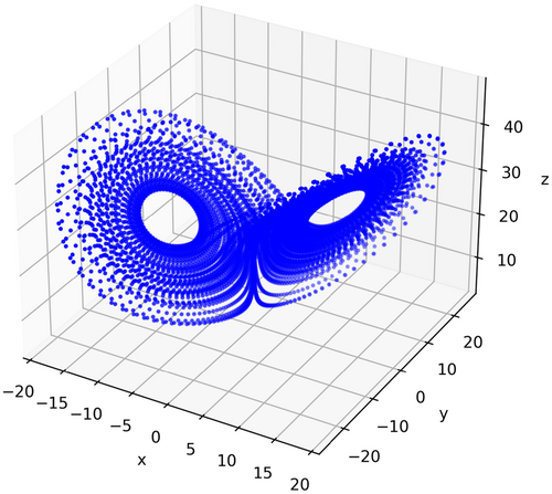
The data used in this study included Lorenz data and streamflow data. The Lorenz data was used for new method verification, while streamflow data was used to further test the effectiveness and stability of the proposed algorithm.

For Lorenz data, it was generated from the Lorenz system, a three-dimensional autonomous system of differential equations:

\{\begin{cases} x' = σ (- x + y) \\ y' = - x z + γ x - y \\ z' = x y - β z \end{cases},

()

where

σ

γ

, and

β

are system parameters. The default selection for system parameters (

σ = 10

γ = 28

β = 8 / 3)

is known to produce a deterministic chaotic time series, which can be presented as a butterfly pattern called the “Lorenz attractor” in Figure 1. The system was solved by the 4-order Runge-Kutta method with a time step of 0.01 s and initial values

x (0) = - 10

y (0) = - 11

z (0) = 47

. A 7000×3 matrix was obtained, and 7000 data points of variable y were selected as the study object.

Details are in the caption following the image — **Figure 1**
Open in figure viewer PowerPoint

Lorenz attractor plot in phase space of variables (x, y, z).

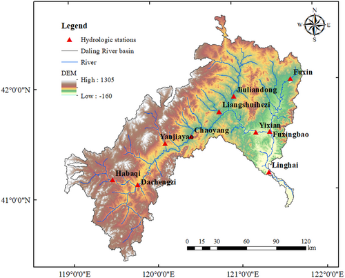
For streamflow data, daily streamflow series in 10 hydrologic stations in the Daling River basin of Liaoning Province, China, which is situated in a semi-arid area with an average annual precipitation of 400–600 mm (as shown in Figure 2), were selected in this study. The start and end dates of these streamflow series are presented in Table 1. It is important to note that, the streamflow data in missing months for Yanjiayao, Liangshuihezi, and Fuxingbao stations in 1997, were substituted with the previous year's data for the same day.

Table 1. Streamflow data series of 10 hydrologic stations in the Daling River basin.

Station number	Station ID	Station name	Start-end of the series (year/month/day)
1	21200355	Dachengzi	1980/1/1–1999/12/31
2	21200450	Chaoyang	1980/1/1–1999/12/31
3	21200600	Yixian	1983/1/1–1999/12/31
4	21200650	Linghai	1980/1/1–1999/12/31
5	21210800	Habaqi	1980/1/1–1999/12/31
6	21211201	Jiuliandong	1980/1/1–1999/12/31
7	21211355	Fuxing	1980/1/1–1999/12/31
8	21210955	Yanjiayao	1980/1/1–1999/12/31
9	21211045	Liangshuihezi	1980/1/1–1999/12/31
10	21211450	Fuxingbao	1980/1/1–1999/12/31

3 RESULTS

3.1 Lorenz data analysis

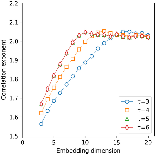
Figure 3 presents the process of calculating correlation exponent with $τ = 6$ and $m = 15$ for the Lorenz attractor based on the proposed algorithm. Based on distinct windows tracking technique, $\log C (r)$ versus $\log r$ curve was divided into 50 segments marked by different colors (Figure 3a). The slope of each segment was determined through the least square fitting of the points within that segment (Figure 3b). The results of fuzzy C-means clustering analysis of these slopes are shown in Figure 3c. It is obvious that the slope exhibited a certain degree of fluctuation, followed by a slightly smaller variation within a specific range, and ultimately infinitely approached 0 at a faster pace. Usually, the second part, represented by red dots, was regarded as the scaling range, and the mean value of the slopes within this range was the correlation exponent we needed. Figure 4 presents the relationship between the correlation exponent and embedding dimension values. The correlation exponent increased with increase in the embedding dimension for $τ$ = 3, 4, 5, 6 up to a certain point and saturated beyond that. The mean saturation value of the correlation exponent (i.e. CD value) was 2.03 ± 0.01, sufficiently close to the theoretical value (i.e., 2.05 ± 0.01) (Grassberger & Procaccia, 1983a), indicating the reasonable effectiveness of the proposed algorithm.

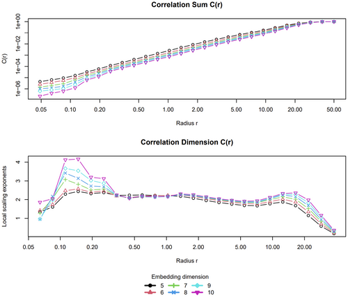
In addition, the package “nonlinearTseries” in R project was employed to detect the CD value of the Lorenz attractor. The time lag and embedding dimension of the Lorenz data were 9 and 5, respectively, and the selected interval of radius (i.e., the scaling region) was from 0.5 to 10. The CD value detected by this package was 2.05 (Figure 5), which was also close to the theoretical value. In summary, the CD values detected by the proposed algorithm and the package “nonlinearTseries” in R project are relatively similar. This indicates that the two methods are both useful to detect the intrinsic dimensionalities of the Lorenz system.

3.2 Actual streamflow data analysis

10 streamflow time series data in the Daling River basin were employed for analysis to further verify the effectiveness of the proposed algorithm. Here, taking the streamflow series of Dachengzi station, Chaoyang station, Yixian station, and Habaqi station, for example, the CD values of four streamflow series were calculated using the proposed algorithm. Figure 6a–d shows the process of calculating the correlation exponent, with specific $τ$ and m for 4 streamflow series of the Daling River basin using the proposed algorithm. Based on the distinct windows tracking technique, $\log C (r)$ versus $\log r$ curve was divided into 50 segments marked by different colors (left figure). The slope of each segment was determined through the least square fitting of the points within that segment (middle figure). The results of fuzzy C-means clustering analysis of these slopes are given in the right figure. As can be seen, the slope showed a certain fluctuation, followed by a rapid decrease, and ultimately infinitely approached 0. Hence, we chose the first part, represented by red dots, as the scaling range. As mentioned above, the mean value of the slopes within this range was the correlation exponent. Figure 7a–d shows the results of the correlation dimension analysis based on the proposed algorithm for 4 streamflow series. For each streamflow series, the correlation exponent, in general, increased with the embedding dimension up to a certain dimension, beyond which it was saturated, for different $τ$ , indicating the presence of deterministic chaos. The CD values of four streamflow series were 3.04, 3.29, 3.16, and 2.56, respectively.

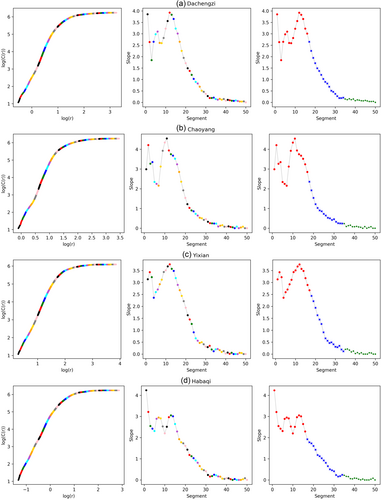
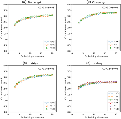
Table 2 provides a summary of the results of correlation dimension analysis performed on all the 10 streamflow time series of Daling River basin based on three methods, including visual inspection method, the proposed method, and the package “nonlinearTseries” in R project. It is worth noting that, in this study, the CD values detected by the visual inspection method, which was combined with the distinct windows tracking technique to improve the accuracy, were considered the true values. The finite non-integer CD values obtained using the proposed algorithm ranged from 2.37 to 3.29, indicating the presence of chaotic behaviors in 10 streamflow series. From Table 2, we can see that the plot of correlation exponent versus embedding dimension of the streamflow series of other hydrologic stations, except Linghai and Jiuliandong stations, saturated for at least three different time lags using the proposed algorithm. This makes the estimated CD values more reliable. In addition, it can be seen that, in most cases, as time lag increases, the embedding dimension may decrease or remain constant.

Table 2. The

τ

, m, and CD values of 10 streamflow series based on three methods.

Name	Visual inspection method			Package “nonlinearTseries”			The proposed method
Name	$τ$	m	CD	$τ$	m	CD	$τ$	m	CD
Dachengzi	5, 6, 8	16, 13, 11	3.19 ± 0.02	5	9	4.07	5, 6, 8	15, 15, 15	3.04 ± 0.03
Chaoyang	5, 6, 7	13, 16, 13	3.85 ± 0.07	3	11	5.93	6, 7, 8	15, 15, 14	3.29 ± 0.01
Yixian	4, 5, 6, 7	16, 15, 12, 11	3.42 ± 0.04	2	14	4.46	6, 7, 8	16, 15, 15	3.16 ± 0.01
Linghai	3, 4, 6	15, 17, 16	2.78 ± 0.23	3	8	2.57	6, 7	19, 17, 15	3.01 ± 0.02
Habaqi	3, 4, 5	11, 8, 8	2.75 ± 0.06	1	10	2.08	3, 4, 5, 6, 7, 8	15, 12, 12, 11, 11, 11	2.56 ± 0.01
Jiuliandong	6, 7, 8	17, 16, 14	2.29 ± 0.11	1	15	0.96	6, 7	18, 17	2.37 ± 0.05
Fuxing	5, 6, 7	15, 12, 12	4.03 ± 0.05	2	12	3.09	3, 4, 5	15, 15, 15	3.18 ± 0.06
Yanjiayao	5, 6, 7	17, 15, 15	3.19 ± 0.04	1	9	2.21	3, 4, 5, 6	15, 16, 17, 17	2.91 ± 0.07
Liangshuihezi	6, 7, 8	17, 17, 16	3.28 ± 0.02	1	13	0.68	4, 6, 7, 8	16, 17, 14, 16	3.08 ± 0.06
Fuxingbao	6, 7, 8	17, 15, 15	3.21 ± 0.02	2	11	2.72	6, 7, 8	17, 15, 15	3.24 ± 0.01

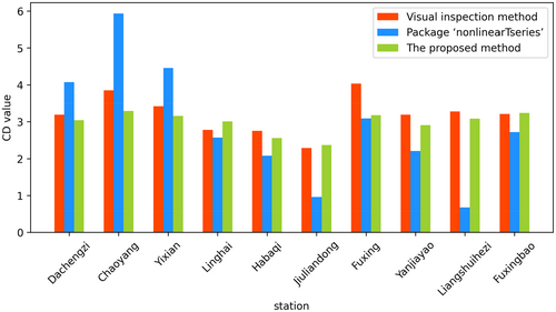
To better compare the results of the correlation dimension analysis based on three methods, the CD values of 10 streamflow series calculated by three methods are shown in Figure 8. It can be observed that, the CD values calculated by the proposed algorithm were closer to the actual CD values than those calculated by the package “nonlinearTseries” in R project. The deviations between the CD values detected by the proposed algorithm and the true values were approximately 0.2 for these streamflow series, except the streamflow series of Chaoyang and Fuxing stations. However, it is evident that there was a significant disparity between the estimated CD values for 10 streamflow series based on the package “nonlinearTseries” and the true values. This indicates it is useful to detect the CD values for the Lorenz data based on the proposed algorithm and the package “nonlinearTseries,” but the proposed algorithm was superior to the package “nonlinearTseries” for the actual streamflow series. Furthermore, to calculate the CD value of one streamflow series with $τ$ from 3 to 8 and $m$ from 3 to 20, the operation time required by the visual inspection method was approximately 3 h, while the proposed method only took 6 min. The average operation efficiency of the proposed algorithm is 30 times faster than that of the visual inspection method (i.e., the original G-P algorithm). In summary, the proposed algorithm is not only intelligent and fast, reducing human interference, but also works better in real-world data.

4 DISCUSSION

As mentioned previously, the results of correlation dimension analysis for the Lorenz data and 10 actual streamflow series based on three methods, including visual inspection method, the proposed method, and the package “nonlinearTseries” in R project, indicate the effectiveness and efficiency of the proposed algorithm for calculating CD values. There was a significant discrepancy between the CD values calculated based on the package “nonlinearTseries” and the true values, primarily due to the following two reasons. First is the choice of time lag and embedding dimension. As we all know, there has always been controversy over the selection of time lag and embedding dimension, which is important for the phase space reconstruction and correlation dimension estimation. Various methods have been proposed for the selection of $τ$ and $m$ , including the autocorrelation function method (e.g., Leung & Lo, 1993), the mutual information method (e.g., Haykin & Puthusserypady, 1997; Haykin & Xiao Bo Li, 1995), the false nearest neighbors (e.g., Hegger et al., 1999; Kennel et al., 1992; Rhodes & Morari, 1997), the correlation integral method (e.g. Ghorbani et al., 2018) and the Cao's method (e.g., Cao, 1997). Different values of $τ$ and $m$ are obtained using different methods, leading to different estimated CD values. In this study, the parameters $τ$ and m involved in correlation dimension analysis based on the package “nonlinearTseries” in R project were obtained using the mutual information method and the Cao's method, respectively, and the estimated CD values differed greatly from the true values. This indicates that it is inaccurate to calculate the CD values by only one $τ$ and only one $m$ . Some studies (e.g., Benmebarek & Chettih, 2023; Di et al., 2018; Di et al., 2019; Labat et al., 2016; Rolim & de Souza Filho, 2023) have selected one $τ$ but multiple $m$ when conducting the correlation dimension analysis. However, it is not reliable, and sometimes, the correlation exponent value increases with an increase in embedding dimension for $τ$ obtained using aforementioned methods. Second is the selection of the scaling region. It is quite difficult and subjective to determine the scaling region of actual data (e.g., streamflow, groundwater, precipitation) by visual inspection method. While it is relatively accurate to detect the CD values based on the visual inspection method combined with the distinct windows tracking technique, it typically requires 3 h for a time series of over 7000 data points. The larger the amount of data, the more time it takes to compute.

In view of these issues, in the present study, different $τ$ and m were tested for each time series, which was a better choice (e.g. Sivakumar, 2000; Tsonis et al., 1993). The CD values were calculated when the saturation range in the correlation exponent versus embedding dimension plot was visible for at least three different time lags. This makes the estimated CD values more stable and convincing. Also, the distinct windows tracking technique, and the fuzzy C-means clustering algorithm, were integrated into the original G-P algorithm. This makes it objective, fast, and accurate to detect the CD value of a chaotic time series, especially actual time series. Nevertheless, there still existed a certain disparity between the estimated CD values obtained using the proposed algorithm and the true values.

Previous studies show that the slope is often not constant within the scaling range for finite real-world data sets (e.g., Sivakumar & Singh, 2012; Sivakumar, 2017), which also can be seen in Figure 5a–d. Thus, it is difficult to identify the scaling region accurately. However, we know the second part, where the slope continuously descended, and the third part, where the slope reached saturation, was definitely not the scaling range, and the first part was considered the scaling range, or at least covered the scaling region. From Figure 6a–d (left), we can find some points did not belong to the linear part, but we were unable to rule them out, leading to the underestimation of the CD values. Further investigations are required to solve this problem in the future.

Additionally, as mentioned above, it is easy to detect the CD values of ideal data, such as the Lorenz data, but it is much more complex to detect the CD values of actual data, such as streamflow, groundwater, and precipitation. In the future, with the continuous extension of actual data length, more time will be required to calculate the CD values. Besides, due to the influence of climate change and anthropogenic activities, the intrinsic dynamic systems of the actual data may change dramatically, leading to large changes in the complexity of the actual data. The choice of study period of actual data also has a certain impact on the CD values. Therefore, it is of great significance to fast and accurately detect the CD values of actual time series. With the development of big data in the future, the proposed algorithm will have stronger generalizability. Before modeling, this algorithm can be used to mine the dimension information, which can greatly reduce the workload and be used to guide the selection of prediction models. This can improve both work efficiency and prediction accuracy to a certain extent. In the future, our research will combine this algorithm with hydrological model simulation and prediction.

5 CONCLUSION

In this study, the distinct windows tracking technique and fuzzy C-means clustering algorithm are introduced in the original G-P algorithm to calculate the correlation dimension value of a chaotic time series. The Lorenz data and streamflow time series data of 10 hydrologic stations in the Daling River basin are employed to verify the effectiveness of the proposed method. Also, the package “nonlinearTseries” in R project is used for comparison. The following conclusions are reached: First, the proposed method is an automatic method for accurately and rapidly calculating the CD values, especially for the actual time series data, and the average operation efficiency of the proposed algorithm is 30 times faster than that of the original G-P algorithm. Second, the CD values of a chaotic time series should be estimated through different time lags and embedding dimensions, which are more reliable than the CD values calculated by only one-time lag and one embedding dimension.

The improved G-P algorithm proposed in this study can fast and accurately detect the CD values of actual time series, such as streamflow, groundwater, and precipitation, thus providing a more reliable estimation of the number of dominant processes of governing the behavior of the time series. It may facilitate a better understanding of complex interactions and feedback behind these actual time series, and provide new insights for the model optimization of these actual time series. Further studies are underway to explore these aspects.

ACKNOWLEDGMENTS

The research was funded by the IWHR Basic Scientific Research Project (JZ110145B0072024), the IWHR Internationally-Oriented Talent for International Academic Leader Program (0203982012), and the National Natural Science Foundation of China (51609257).

ETHICS STATEMENT

None declared.

APPENDIX A: Package “nonlinearTseries”

Package “nonlinearTseries” was developed by Constantino A. Garcia and Gunther Sawitzk. It depends on R greater than or equal to version 3.3.0. It can be downloaded from https://github.com/constantino-garcia/nonlinearTseries. This package permits the computation of the most-used nonlinear statistics/algorithms, including generalized correlation dimension, information dimension, largest Lyapunov exponent, sample entropy, and Recurrence Quantification Analysis (RQA), among others.

Open Research

DATA AVAILABILITY STATEMENT

The data that support the findings of this study are available from the corresponding author upon reasonable request.

REFERENCES

Benmebarek, S., & Chettih, M. (2023). Chaotic analysis of daily runoff time series using dynamic, metric, and topological approaches. Acta Geophysica, 72, 2633–2651.
10.1007/s11600-023-01150-0
Web of Science® Google Scholar
Bezdek, J. C. (1981). Objective function clustering (pp. 43–93). Springer.
10.1007/978-1-4757-0450-1_3
Google Scholar
Bezdek, J. C., Ehrlich, R., & Full, W. (1984). FCM: The fuzzy c-means clustering algorithm. Computers & Geosciences, 10, 191–203.
10.1016/0098-3004(84)90020-7
Web of Science® Google Scholar
Bolea, J., Laguna, P., Remartínez, J. M., Rovira, E., Navarro, A., & Bailón, R. (2014). Methodological framework for estimating the correlation dimension in HRV signals. Computational and Mathematical Methods in Medicine, 2014(1), 1–11.
10.1155/2014/129248
Google Scholar
Camastra, F., Esposito, F., & Staiano, A. (2018). Linear SVM-based recognition of elementary juggling movements using correlation dimension of Euler Angles of a single arm. Neural Computing and Applications, 29, 1005–1013.
10.1007/s00521-016-2616-x
Web of Science® Google Scholar
Cao, L. (1997). Practical method for determining the minimum embedding dimension of a scalar time series. Physica D: Nonlinear Phenomena, 110(1–2), 43–50.
10.1016/S0167-2789(97)00118-8
Web of Science® Google Scholar
Chen, Z., Liu, Y., & Zhou, P. (2019). A novel method to identify the scaling region of rough surface profile. Fractals, 27(2), 1950011.
10.1142/S0218348X19500117
Web of Science® Google Scholar
Corana, A. (2000). Adaptive box-assisted algorithm for correlation-dimension estimation. Physical Review E, 62, 7872–7881.
10.1103/PhysRevE.62.7872
CAS Web of Science® Google Scholar
Dang, J. W., & Huang, J. G. (2004). Study of the parameters used in calculating correlative dimension based on G.P algorithm. Computer Application Research, 21(1), 48–51in Chinese.
Google Scholar
Decoster, G. P., & Mitchell, D. W. (1991). The efficacy of the correlation dimension technique in detecting determinism in small samples. Journal of Statistical Computation and Simulation, 39, 221–229.
10.1080/00949659108811357
Google Scholar
Di, C., Wang, T., Han, Q., Mai, M., Wang, L., & Chen, X. (2023). Complexity and predictability of daily actual evapotranspiration across climate regimes. Water Resources Research, 59, 4.
10.1029/2022WR032811
Web of Science® Google Scholar
Di, C., Wang, T., Istanbulluoglu, E., Jayawardena, A. W., Li, S., & Chen, X. (2019). Deterministic chaotic dynamics in soil moisture across Nebraska. Journal of Hydrology, 578, 124048.
10.1016/j.jhydrol.2019.124048
Web of Science® Google Scholar
Di, C. L., Wang, T. J., Yang, X. H., & Li, S. L. (2018). Technical note: An improved grassberger–procaccia algorithm for analysis of climate system complexity. Hydrology & Earth System Sciences, 22(10), 5069–5079.
10.5194/hess-22-5069-2018
Web of Science® Google Scholar
Du, B. Q., Jia, Z. W., & Tang, G. J. (2013). A new identification method for fractal scaling region of a vibration signal (in Chinese). Journal of Vibration and Shock, 32(14), 40–45.
Google Scholar
Dunn, J. C. (1973). A fuzzy relative of the ISODATA process and its use in detecting compact well-separated clusters. Journal of Cybernetics, 3, 32–57.
10.1080/01969727308546046
Web of Science® Google Scholar
Ghorbani, M. A., Khatibi, R., Danandeh Mehr, A., & Asadi, H. (2018). Chaos-based multigene genetic programming: A new hybrid strategy for river flow forecasting. Journal of Hydrology, 562, 455–467.
10.1016/j.jhydrol.2018.04.054
Web of Science® Google Scholar
Grassberger, P. (1990). An optimized box-assisted algorithm for fractal dimensions. Physics Letters A, 148, 63–68.
10.1016/0375-9601(90)90577-B
Web of Science® Google Scholar
Grassberger, P., & Procaccia, I. (1983a). Characterization of strange attractors. Physical Review Letters, 50, 346–349.
10.1103/PhysRevLett.50.346
Web of Science® Google Scholar
Grassberger, P., & Procaccia, I. (1983b). Measuring the strangeness of strange attractors. Physica D, 9, 189–208.
10.1016/0167-2789(83)90298-1
Web of Science® Google Scholar
Harikrishnan, K. P., Misra, R., Ambika, G., & Kembhavi, A. K. (2006). A non-subjective approach to the GP algorithm for analysing noisy time series. Physica D: Nonlinear Phenomena, 215(2), 137–145.
10.1016/j.physd.2006.01.027
Web of Science® Google Scholar
Haykin, S., & Puthusserypady, S. (1997). Chaotic dynamics of sea clutter. Chaos: An Interdisciplinary Journal of Nonlinear Science, 7(4), 777–802.
10.1063/1.166275
Google Scholar
Haykin, S., & Xiao Bo Li. (1995). Detection of signals in chaos. Proceedings of the IEEE, 83(1), 95–122.
10.1109/5.362751
Web of Science® Google Scholar
Hegger, R., Kantz, H., & Schreiber, T. (1999). Practical implementation of nonlinear time series methods: The TISEAN package. Chaos: An Interdisciplinary Journal of Nonlinear Science, 9, 413–435.
10.1063/1.166424
Web of Science® Google Scholar
Huang, F., Ochoa, C. G., Guo, L. D., Wu, Y., & Qian, B. (2020). Investigating variation characteristics and driving forces of lake water level complexity in a complex river-lake system. Stochastic Environmental Research and Risk Assessment, 8, 1–15.
Google Scholar
Ji, C., Zhu, H., & Jiang, W. (2011). A novel method to identify the scaling region for chaotic time series correlation dimension calculation. Chinese Science Bulletin, 56(9), 925–932.
10.1007/s11434-010-4180-6
Web of Science® Google Scholar
Jia, Z. W., Wang, P., & Fang, J. Y. (2012). Fractal scaleless band automatic identification for fractal theory application (in Chinese). Machinery, 39(11), 24–26+30.
Google Scholar
Jothiprakash, V., & Fathima, T. A. (2013). Chaotic analysis of daily rainfall series in Koyna reservoir catchment area, India. Stochastic Environmental Research and Risk Assessment, 27, 1371–1381.
10.1007/s00477-012-0673-y
Web of Science® Google Scholar
Judd, K. (1994). Estimating dimension from small samples. Physica D: Nonlinear Phenomena, 71(4), 421–429.
10.1016/0167-2789(94)90008-6
Google Scholar
Kennel, M. B., Brown, R., & Abarbanel, H. D. I. (1992). Determining embedding dimension for phase-space reconstruction using a geometrical construction. Physical Review A, 45(6), 3403–3411.
10.1103/PhysRevA.45.3403
CAS PubMed Web of Science® Google Scholar
Kim, H. S., Eykholt, R., & Salas, J. D. (1999). Nonlinear dynamics, delay times, and embedding windows. Physica D: Nonlinear Phenomena, 127(1–2), 48–60.
10.1016/S0167-2789(98)00240-1
Web of Science® Google Scholar
Labat, D., Sivakumar, B., & Mangin, A. (2016). Evidence for deterministic chaos in long-term high-resolution karstic streamflow time series. Stochastic Environmental Research and Risk Assessment, 30(8), 2189–2196.
10.1007/s00477-015-1175-5
Web of Science® Google Scholar
Leung, H., & Lo, T. (1993). Chaotic radar signal processing over the sea. IEEE Journal of Oceanic Engineering, 18(3), 287–295.
10.1109/JOE.1993.236367
Web of Science® Google Scholar
Maragos, P., & Fan-Kon sun, S. (1993). Measuring the fractal dimension of signals. IEEE Transactions on Signal Processing, 41, 108–121.
10.1109/TSP.1993.193131
Web of Science® Google Scholar
Mcmahon, C. J., Toomey, J. P., & Kane, D. M. (2017). Insights on correlation dimension from dynamics mapping of three experimental nonlinear laser systems. PLoS One, 12, e0181559.
10.1371/journal.pone.0181559
PubMed Web of Science® Google Scholar
Ogunjo, S., Akinsusi, J., Rabiu, B., & Fuwape, I. (2024). Dynamical complexity and multifractal analysis of geomagnetic activities at high temporal scales over three solar cycles. Journal of Atmospheric and Solar-Terrestrial Physics, 265, 106380.
10.1016/j.jastp.2024.106380
Web of Science® Google Scholar
Rhodes, C., & Morari, M. (1997). The false nearest neighbor algorithm: An overview. Computers & Chemical Engineering, 21, 1149–1154.
10.1016/S0098-1354(97)00204-4
Google Scholar
Rolim, L. Z. R., & de Souza Filho, F. A. (2023). Exploring spatiotemporal chaos in hydrological data: Evidence from Ceará, Brazil. Stochastic Environmental Research and Risk Assessment, 37(11), 4513–4537.
10.1007/s00477-023-02501-5
Web of Science® Google Scholar
Shen, S., Song, C., Cheng, C., & Ye, S. (2020). The coupling impact of climate change on streamflow complexity in the headwater area of the northeastern Tibetan Plateau across multiple timescales. Journal of Hydrology, 588, 124996.
10.1016/j.jhydrol.2020.124996
Web of Science® Google Scholar
Shu, Z. R., Chan, P. W., Li, Q. S., He, X. H., & Cai, C. Z. (2023). Characterising the variability in ocean data using fractal and correlation dimension analysis. Applied Ocean Research, 138, 103590.
10.1016/j.apor.2023.103590
Web of Science® Google Scholar
Sivakumar, B. (2000). Chaos theory in hydrology: Important issues and interpretations. Journal of Hydrology, 227, 1–20.
10.1016/S0022-1694(99)00186-9
Web of Science® Google Scholar
Sivakumar, B. (2004a). Chaos theory in geophysics: Past, present and future. Chaos, Solitons, and Fractals, 19, 441–462.
10.1016/S0960-0779(03)00055-9
Web of Science® Google Scholar
Sivakumar, B. (2017). Chaos in hydrology: Bridging determinism and stochasticity. Springer.
10.1007/978-90-481-2552-4
Google Scholar
Sivakumar, B., & Singh, V. P. (2012). Hydrologic system complexity and nonlinear dynamic concepts for a catchment classification framework. Hydrology and Earth System Sciences, 16, 4119–4131.
10.5194/hess-16-4119-2012
Web of Science® Google Scholar
Takens, F. (1981). Detecting strange attractors in turbulence, Dynamical systems and turbulence, Warwick 1980 (pp. 366–381). Springer.
10.1007/BFb0091924
Google Scholar
Tang, L., Lv, H., Yang, F., & Yu, L. (2015). Complexity testing techniques for time series data: A comprehensive literature review. Chaos, Solitons & Fractals, 81, 117–135.
10.1016/j.chaos.2015.09.002
Web of Science® Google Scholar
Theiler, J. (1987). Efficient algorithm for estimating the correlation dimension from a set of discrete points. Physical Review A, 36, 4456–4462.
10.1103/PhysRevA.36.4456
CAS PubMed Web of Science® Google Scholar
Toledo, E., Toledo, S., Almog, Y., & Akselrod, S. (1997). A vectorized algorithm for correlation dimension estimation. Physics Letters A, 229(6), 375–378.
10.1016/S0375-9601(97)00186-2
CAS Web of Science® Google Scholar
Tsonis, A. A., Elsner, J. B., & Georgakakos, K. P. (1993). Estimating the dimension of weather and climate attractors: Important issues about the procedure and interpretation. Journal of the Atmospheric Sciences, 50, 2549–2555.
10.1175/1520-0469(1993)050<2549:ETDOWA>2.0.CO;2
Web of Science® Google Scholar
Wang, F. Q., Luo, C. S., & Chen, G. X. (1993). An improvement of G-P algorithm and its application (in Chinese). Physica D: Computational Physics, 10(3), 345–351.
Google Scholar
Wang, Y., Tao, Y., Sheng, D., Zhou, Y., Wang, D., Shi, X., Wu, J., & Ma, X. (2020). Quantifying the change in streamflow complexity in the Yangtze River. Environmental Research, 180, 108833.
10.1016/j.envres.2019.108833
CAS PubMed Web of Science® Google Scholar
Wu, H. S., Ni, L. P., Zhang, F. M., Zhou, X., & Du, J. Y. (2014). A method for calculating fractal dimension of multivariable time series (in Chinese). Control and Decision, 29(3), 455–459.
Google Scholar
Wu, Z. C. (2002). Determination of fractal scaleless range (in Chinese). Acta Geotechnica et Cartographica Sinica, 31(3), 240–244.
Google Scholar
Yang, H. Y., Ye, H., Wang, G. Z., & Pan, G. D. (2008). Identification of scaling regime in chaotic correlation dimension calculation. 2008 3rd IEEE Conference on Industrial Electronics and Applications. IEEE.
Google Scholar
Yokoya, N., & Yamatomo, K. (1989). Fractal-based analysis and interpolation of 3D natural surfaces and their applications to terrain modeling. CVGIP, 46, 284–302.
Google Scholar
Zhou, S., Wang, X., Zhou, W., & Zhang, C. (2022). Recognition of the scale-free interval for calculating the correlation dimension using machine learning from chaotic time series. Physica A: Statistical Mechanics and its Applications, 588, 126563.
10.1016/j.physa.2021.126563
Web of Science® Google Scholar

Volume4, Issue2

May 2025

Pages 253-264

An intelligent algorithm to fast and accurately detect chaotic correlation dimension

Abstract

1 INTRODUCTION