Robust adaptive model predictive control: Performance and parameter estimation

1 INTRODUCTION

Model predictive control (MPC) repeatedly solves a finite-horizon optimal control problem subject to input and state constraints. At each sampling instant a model of the plant is used to optimize predicted behavior and the first element of the optimal predicted control sequence is applied to the plant.¹ Any mismatch between model and plant causes degradation of controller performance.² As a result, the amount of model uncertainty strongly affects the bounds of the achievable performance of a robust MPC algorithm.³

To avoid the disruption caused by intrusive plant tests,² adaptive MPC attempts to improve model accuracy online while satisfying operating constraints and providing stability guarantees. Although the literature on adaptive control has long acknowledged the need for persistently exciting (PE) inputs for system identification,⁴ few articles have explored how to incorporate PE conditions with feasibility guarantees within adaptive MPC.⁵ In addition, adaptive MPC algorithms must balance conflicting requirements for system identification accuracy and computational complexity.^{5, 6}

Various methods for estimating system parameters and meeting operating constraints are described in the adaptive MPC literature. Depending on the assumptions on model parameters, parameter identification methods such as recursive least squares (RLS)⁷, comparison sets,⁸ set membership identification,^{9, 10} and neural networks^{11, 12} have been proposed. Heirung et al¹³ propose an algorithm where the unknown parameters are estimated using RLS and system outputs are predicted using the resulting parameter estimates. The use of RLS introduces nonlinear equality constraints into the optimization. On the other hand, the comparison model approach described in Aswani et al⁸ addresses the trade-off between probing for information and output regulation by decoupling these two tasks; a nominal model is used to impose operating constraints whereas performance is evaluated via a model learned online using statistical identification tools. However, the use of a nominal model implies that the comparison model approach cannot guarantee robust constraint satisfaction.

Tanaskovic et al⁹ consider a linear finite impulse response (FIR) model with measurement noise and constraints. This approach updates a model parameter set using online set membership identification; constraints are enforced for the entire parameter set and performance is optimized for a nominal prediction model. The article proves recursive feasibility but does not show convergence of the identified parameter set to the true parameters. To avoid the restriction to FIR models, Lorenzen et al¹⁰ consider a linear state space model with additive disturbance. An online-identified set of possible model parameters is used to robustly stabilize the system. However, the approach suffers from a lack of flexibility in its robust MPC formulation, which is based on homothetic tubes,¹⁴ allowing only the centers and scalings of tube cross-sections to be optimized online, and it does not provide convex and recursively feasible conditions to ensure PE control inputs.

In this article, we also consider linear systems with parameter uncertainty, additive disturbances, and constraints on system states and control inputs. Compared with Reference 10, the proposed algorithm reduces the conservativeness in approximating predicted state tubes by adopting more flexible cross-section representations. Building on Reference 15, we take advantage of fixed complexity polytopic tube representations and use hyperplane and vertex representations interchangeably to further simplify computation. We use, similarly to Reference 13, a nominal performance objective, but we impose constraints robustly on all possible models within the identified model set. We prove that the closed-loop system is input-to-state stable (ISS). In comparison with the min-max approach of Reference 15, the resulting performance bound takes the form of an asymptotic bound on the 2-norm of the sequence of closed-loop states in terms of the 2-norms of the additive disturbance and parameter estimate error sequences. In addition, we convexify the persistence of excitation (PE) condition around a reference trajectory and include a penalty term in the cost function to promote convergence of the parameter set. The convexification method is somewhat analogous to that proposed in References 16, 17, where the uncertainty information of the parameter set is approximated using a nominal gain. Here, however, the convexification is obtained by direct linearization of PE constraints on predicted trajectories. The cost function modification proposed here allows the relative importance of the two objectives, namely, controller performance and convergence of model parameters, to be specified.

Bai et al¹⁸ consider a particular set membership identification algorithm and show that the parameter set estimate converges with probability 1 to the actual parameter vector (assumed constant) if: (a) a tight bound on disturbances is known; (b) the input sequence is persistent exciting; and (c) the minimal parameter set estimate is employed. However, the minimal set estimate can be arbitrarily complex, and to provide computational tractability various nonminimal parameter set approximations have been proposed, such as n-dimensional balls¹⁹ and bounded complexity polytopes.⁹ The current article allows the use of parameter set estimates with fixed complexity and proves that, despite their approximate nature, such parameter sets converge with probability 1 to the true parameter values. We also derive lower bounds on convergence rates for the case of inexact knowledge of the disturbance bounding set and for the case that model states are estimated in the presence of measurement noise.

This article has five main parts. Section 2 defines the problem and basic assumptions. Section 3 gives details of the parameter estimation, robust constraint satisfaction, nominal cost function, convexified PE conditions, and the MPC algorithm. Section 4 proves recursive feasibility and ISS of the proposed algorithm. Section 5 proves the convergence of the parameter set in various conditions and Section 6 illustrates the approach with numerical examples.

Notation: and denote the sets of integers and reals, and , . The ith row of a matrix A and ith element of a vector a are denoted [A]_i and [a]_i. Vectors and matrices of 1s are denoted 1, and is the identity matrix. For a vector a, ‖a‖ is the Euclidean norm and ; the largest element of a is and . The absolute value of a scalar s is and the floor value is ⌊s⌋. is the number of elements in a set . is Minkowski addition for sets and , and . The matrix inequality A ≽ 0 (or A ≻ 0) indicates that A is positive semidefinite (positive definite) matrix. The k steps ahead predicted value of a variable x is denoted x_k, and the more complete notation x_k|t indicates the k steps ahead prediction at time t. A continuous function is a -function if it is strictly increasing with , and is a -function if in addition as s → ∞. A continuous function is a -function if, for all t ≥ 0, is a -function, and, for all s ≥ 0, is decreasing with as t → ∞. For functions and we denote , and with .

2 PROBLEM FORMULATION AND PRELIMINARIES

This article considers a linear system with linear state and input constraints and unknown additive disturbance:

(1)

where is the system state, is the control input, is an unknown disturbance input, and t is the discrete time index. The system matrices and depend on an unknown but constant parameter . The disturbance sequence {w₀,w₁, …} is stochastic and (w_i,w_j) is independent for all i ≠ j. States and control inputs are subject to linear constraints, defined for , by

(2)

Assumption 1. (Additive disturbance)The disturbance w_t lies in a convex and compact polytope , where

(3)

with , and .

Assumption 2. (Parameter uncertainty)The system matrices A and B are affine functions of the parameter vector :

(4)

for known matrices A_j, B_j, , and lies in a known, bounded, convex polytope given by

Assumption 3. (State and control constraints)The set

is compact and contains the origin in its interior.

To obtain finite numbers of decision variables and constraints in the MPC optimization problem, the predicted control sequence at time t is assumed to be expressed in terms of optimization variables v_0|t, … , v_{N − 1|t} as

(5)

where N is the prediction horizon. The gain K is designed offline and is assumed to robustly stabilize the uncertain system , in the absence of constraints. This assumption can be stated as follows.

Assumption 4. (Feedback gain and contractive set)There exists a polytopic set and feedback gain K such that is -contractive for some , that is

(6)

for all x ∈ {x : Tx ≤ 1} and . The representation is assumed to be minimal in the sense that it contains no redundant inequalities.

3 ADAPTIVE ROBUST MPC

In this section, a parameter estimation scheme based on References 20, 21 is introduced. We then discuss the construction of tubes to bound predicted model states and associated constraints.

3.1 Set-based parameter estimation

At time t we use observations of the system state x_t to determine a set of unfalsified model parameters. The set is then combined with the parameter set estimate to construct a new parameter set estimate .

Unfalsified parameter set: Define D_t and d_t as the matrix and vector

(7)

(8)

Then, given x_t, x_t − 1, u_t − 1 and the disturbance set in (3), the unfalsified parameter set at time t is given by

(9)

with and .

Parameter set update: Let be an a priori chosen matrix. The estimated parameter set is defined by

(10)

where is updated online at times . The complexity of is controlled by fixing , which fixes the directions of the half-spaces defining the parameter set. We assume that is chosen so that is compact for all such that . Using a block recursive polytopic update method,²⁰ is defined as the smallest set (10) containing the intersection of and unfalsified sets over a window of length N_u:

(11)

(where for all j ≤ 0). We refer to N_u as the PE window. Note that N_u is independent of the MPC prediction horizon N. Using linear conditions for polyhedral set inclusion²² in (11) can be obtained by solving a linear program for each :

Lemma 1.If and is defined by (10), (11), then and for all .

3.2 Polytopic tubes for robust constraint satisfaction

This section considers predicted state and control trajectories. To simplify notation, we omit the subscript t indicating the time at which state and control predictions are made, whenever t indicates current time; thus the k steps ahead predictions x_k|t, v_k|t are denoted x_k, v_k. To ensure that the predicted state and control sequences satisfy the operating constraints (2) robustly for the given uncertainty bounds, we construct a tube (a sequence of sets) satisfying, for all , , ,

(12)

Hyperplane form: For given satisfying Assumption 4 and , let denote the k steps ahead cross-section of the predicted state tube:

(13)

The MPC algorithm described in Section 3.5 optimizes the shape of the predicted state tube online by allowing to be an optimization variable. If, for a given , the constraint is redundant for some in the hyperplane description (13) (ie, if the set is unchanged by removing this constraint), we define (without loss of generality) . Thus, for each , necessarily holds for some . Then (12) is equivalent to, for all and ,

where is the vector with ith element for all . Substituting D(x,u) and d(x,u) from (7), (8), this implies linear conditions on , for all , :

and, for a given initial state x, the constraint requires

(14)

Vertex form:  has an equivalent representation in terms of its vertices, which we denote as , :

(15)

Note that m, the number of vertices of , is fixed, and for given in (13), we may have for some in (15) (ie, the vertex description may contain repeated vertices). The presence of repeated vertices does not affect the formulation. For each , define an index set (with ), such that the ith row of T and ith element of satisfy

Since T is constant, the index set associated with active inequalities at the vertex x^(j) is independent of and can be computed offline. Therefore, for each , we have

(16)

where the matrix can be computed offline given knowledge of using the property that

(17)

Using the vertex representation (16), the condition that (2) is satisfied for all is equivalent to, for all ,

(18)

Substituting D(x,u) and d(x,u) from (7), (8), condition (12) can be expressed equivalently as

for all , and . This is equivalent (see e.g. Reference 22, Proposition 3.31) to the requirement that there exist matrices satisfying, for each prediction time step and each vertex , the conditions

(19a)

(19b)

(19c)

Given the dual mode predicted control law (5), we introduce the terminal conditions that and (F + GK)x ≤ 1 for all , , and . Then (2) and (12) are satisfied if (18), (19) hold for all and , and there exist matrices satisfying the conditions, for all

(20a)

(20b)

(20c)

(20d)

3.3 Objective function

Consider the nominal cost defined for Q, R ≻ 0 by

(21)

where and are elements of predicted state and control sequences generated by a nominal parameter vector :

(22a)

(22b)

(22c)

for and where v = {v₀, … , v_N − 1}. Define as the solution of the Lyapunov matrix equation

(23)

where . Note that is well-defined for all due to Assumption 4. Then (21) is equivalent to

(24)

We assume knowledge of an initial nominal parameter vector , which could be estimated using physical modeling or offline system identification, alternatively could be defined as the Chebyshev center of . For t > 0, we assume that is updated by projecting onto the parameter set estimate , that is

(25)

Remark 1.For the ISS analysis in Section 4 it is essential that . However, subject to this constraint, alternative update laws for are possible; for example, a least mean squares estimate projected onto .¹⁰

3.4 Augmented objective function and persistent excitation

The regressor D_t in (7) is PE if

(26)

for some PE window , some , and all times t₀.⁴ Although the upper bound in (26) implies convex constraints on x_t and u_t, the lower bound is nonconvex. The bounds on convergence of the parameter set derived in Section 5 suggest faster convergence as in the PE condition (26) increases.

Previously proposed MPC strategies that incorporate PE constraints consider the PE condition to be defined on an interval such as {t − N_u + 1, … , t}, where t is current time, which means that the PE constraint depends on only the first element of the predicted control sequence. Marafioti et al²³ simplify the PE condition by expressing it as a nonconvex quadratic inequality in u_t. Likewise, Lorenzen et al¹⁰ show that the PE condition is equivalent to a nonconvex constraint on the current control input. Lu and Cannon¹⁵ linearize the PE condition about a reference trajectory and thus obtain a sufficient condition for persistent excitation.

In this article, on the hand, we define the PE condition over predicted trajectories (from k = 0 to k = N_u − 1 steps ahead), and we therefore require, at time t and for some ,

(27)

The inclusion of predicted future states and control inputs in this PE condition allows for greater flexibility in meeting the constraint. To avoid nonconvex constraints, we derive a convex relaxation that provides a sufficient condition for (27).

Assume reference state and control predicted sequences, and , approximating the optimal predicted state and control sequences, are available. To derive sufficient conditions for (27), we consider the difference between the reference and optimized sequences, denoted and (ie, and ). Since the prediction tube implies , we therefore have where . Denote the vertices of as and for , we have

Moreover, D_k depends linearly on u_k and x_k, and hence for ,

Here, is a positive semidefinite matrix, and by omitting this term we obtain sufficient conditions for (27) as a set of LMIs in and v_k. The following convex conditions are thus sufficient to ensure (27) whenever

(28a)

(28b)

where are intermediate variables.

Another innovation of this article is the inclusion of PE coefficient in the cost function. Previous approaches^{10, 15} face the difficulty of choosing a suitable value for the PE constraint in the implementation. A larger value of is generally desirable, but a large might make the optimization problem with the PE condition infeasible. In this article, we incentivize a large value of by modifying the MPC objective function as follows

(29)

where is a weight that controls the relative priority given to satisfaction of the PE condition (27) and tracking performance. This modification does not affect the feasibility of the optimization.

Although incorporating a condition such as (27) or the convex relaxation (28) and (29) into a MPC strategy does not ensure that the closed-loop system satisfies a corresponding PE condition, its effect on the convergence rate of the estimated parameter set is significant, as shown in the numerical example in Section 6. In addition, is a meaningful and straightforward coefficient to tune, and the PE constraint can be easily switched off by setting .

3.5 Proposed algorithm

Offline:

• 1. Choose suitable T defining the predicted state tube and compute the corresponding U_j in (17).
• 2. Obtain a nominal .
• 3. Minimize the contracitivity factor satisfying (6) and obtain a feedback gain K.

Online: For t = 0,1,2,…

• 1. Obtain the current state x_t and set x = x_t.
• 2. Update using (11) and the nominal parameter vector using (25), and solve (23) for .
• 3.

  At t = 0 compute the initial reference state and control sequences and , for example, by solving the nominal problem described in Remark 4.

  At t > 0 compute the reference state and control sequences and , using the solution at t − 1, and

  (30)

• 4. Compute , , , , , the solution of the semidefinite program (SDP):
  
• 5. Implement the current control input .

Remark 2.In offline step 1, T can be chosen so that the polytope in Assumption 4 approximates a robust control invariant set of the form , where satisfies for some . Using the vertex representation of , the matrix can be computed by solving a SDP (see e.g. Reference 24, Chapter 5). This approach allows the number of rows in T to be specified by the designer. However, T can alternatively be chosen so that approximates the minimal robust positive invariant (RPI) set or the maximal RPI set for the system (1) and (2) under a specified stabilizing feedback law.²²

Remark 3.In offline step 3, the computation of subject to (6) for given T can be performed by solving a LP using the vertex representation of  [ 22, chap. 7]. The objective of minimizing is chosen to make the constraints of problem  easier to satisfy. In particular, choosing K so that in (6) ensures that exists satisfying the terminal constraints (20b-d).

Remark 4.At t = 0, the reference sequences and may be computed by solving

(31)

Remark 5.The online computation of the proposed algorithm may be reduced by updating only once every N_u > 1 time steps. For example, in Step 2, set for t ∈ {N_u,2N_u, …} and at all times t ∉ {N_u,2N_u, …}.

In Section 4, we use the property that to show that the solution, , of at time t − 1 forms part of a feasible solution of at time t. As a result, the reference sequences , in Step 3 are feasible for problem at all times t > 0.

4 RECURSIVE FEASIBILITY AND STABILITY

4.1 Recursive feasibility

At time t ≥ 1, let a suboptimal set of decision variables, denoted be defined in terms of the optimal solution of at time t − 1 by

Proposition 1. (Recursive Feasibility)The online MPC optimization is feasible at all times if is feasible at t = 0 and for all time t.

Proof.If is feasible at t − 1, then at time t, is: feasible for (14) because ; feasible for (18) and (19) for because is feasible for (18) and (19) for and ; and feasible for (18) and (19) for k = N − 1 and feasible for (20) because is feasible for (20) and . Finally, we note that (22) is necessarily feasible and (28) necessarily holds for some scalar if .

4.2 Input-to-state stability

Throughout this section we set in problem . Therefore, the objective of is where J is the nominal cost (24). As a result of parameter adaption, the change of online might increase the cost, but this is absorbed in the ISS terms. To simplify notation we define a stage cost L(x,v) and terminal cost as and so that (24) is equivalent to

Denoting the actual state at next time step as x⁺, we define the function as

so that .

Lemma 2. (ISS-Lyapunov function [25])The system

(32)

with control law is ISS with region of attraction if the following conditions are satisfied.

(i).  contains the origin in its interior, is compact, and is a robust positively invariant set for (32), that is, for all , , , and .

(ii). There exist - functions , -functions , and a function such that for all , is continuous, and for all ,

(33)

(34)

In the following, we define as the set of states x such that problem is feasible and assume that is nonempty. In addition, for a given state x, nominal parameter vector , and parameter set , we denote as the optimal solution of problem , and let be the corresponding optimal value of the cost in (24), so that .

Theorem 1.Assume that and the nominal parameter vector is not updated, that is,  for all . Then for all initial conditions , the system (1) with control law , where is the first element of , robustly satisfies the constraint (2) and is ISS with region of attraction .

Proof.We first show that condition (i) of Lemma 2 is satisfied with . If is feasible at t = 0, then (20) implies that exists such that satisfies

(35)

Therefore is feasible for for all , and hence . In addition, the robust invariance of implied by (35) ensures that , and since due to Assumption 1, must contain the origin in its interior. Furthermore, Proposition 1 shows that if is initially feasible, then it is feasible for all t ≥ 0, so that is positively invariant for (32). Finally, is necessarily compact by Assumption 3, and it follows that condition (i) of Lemma 2 is satisfied if .

We next consider the bounds (33) in condition (ii) of Lemma 2. For a given state x, nominal parameter vector and parameter set , problem with and Q, R ≻ 0 is a convex quadratic program. Therefore, is a continuous positive definite, piecewise quadratic function of x²⁶ for each and . Furthermore, is compact due to Assumption 2 and it follows that there exist -functions , such that (33) holds with

To show that the bound (34) in condition (ii) of Lemma 2 holds, let denote the set . Then, given the linear dependence of the system (1), the model parameterization (4), and the predicted control law (5) on the state x, disturbance w, and parameter vector , and since , , , and are compact sets by Assumptions 1,2, and 3, there exist functions , , , , such that, , , , ,

Following the proof of Theorem 5 in Limon et al²⁵ and using the weak triangle inequality for -functions,²⁷ we obtain

where and 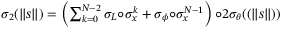, and both and are -functions. Since is a feasible but suboptimal solution of at x⁺, and since by assumption, the optimal cost function satisfies and hence

Thus, all conditions of Lemma 2 are satisfied.

Corollary 1.Assume that and the nominal parameter vector is updated at each time using (25). Then for all initial conditions , the system (1) with control law , where is the first element of , robustly satisfies the constraint (2) and is ISS with region of attraction .

Proof.It can be shown that condition (i) of Lemma 2 and the bounds (33) in condition (ii) of Lemma 2 are satisfied with and for some -functions , using the same argument as the proof of Theorem 1. To show that (34) is also satisfied and hence complete the proof we use an argument similar to the proof of Theorem 1. In particular, as before we define using the optimal solution of , , and

However, here we define z = {z₀, … , z_N} as the sequence

where has for and . Then implies

(36)

The update law (25) ensures that since . Hence, for all , we have

and it follows that, for all ,

where . In addition we have, for all

and, since Q ≻ 0, there exists a function such that , while (23) implies

Furthermore (23) is linear in and the solution is unique for all (see, eg, Reference 28) since is by assumption stable. Therefore, by the implicit function theorem, is Lipschitz continuous and for all , , for some . Hence

Collecting the bounds derived above on individual terms in the expression for in (36), we obtain

where , are -functions. But by optimality we have . Therefore (34) holds and hence all of the conditions of Lemma 2 are satisfied.

Remark 6.The ISS property implies that there exists a -function and -functions and such that for all feasible initial conditions , the closed-loop system trajectories satisfy, for all ,

Remark 7.Theorem 1 and Corollary 1 do not apply to the case that . However, if is replaced by a time-varying weight in the objective of problem , then ISS can be guaranteed by setting for all t ≥ t₀, for some finite horizon t₀.

5 CONVERGENCE OF THE ESTIMATED PARAMETER SET

In terms of D and d defined in (7) and (8), the system model can be rewritten as

(37)

where x_t + 1, D(x_t,u_t), and d(x_t,u_t) are known at time t + 1. Thus, the system is linear with regressor D_t, uncertain parameter vector , and additive disturbance .

Bai et al¹⁸ show that, for such a system, the diameter of the parameter set constructed using a set-membership identification method converges to zero with probability 1 if the uncertainty bound is tight and the regressor D_t is PE. We extend this result and prove convergence of the estimated parameter set in more general cases. Specifically, in this article we avoid the problem of computational intractability arising from a minimum volume update law of the form . Instead, we derive stochastic convergence results for parameter sets with fixed complexity and update laws of the form .

In this section, we first discuss relevant results for an update law that gives a minimal parameter set estimate for a given sequence of states (but whose representation has potentially unbounded complexity), before considering convergence of the fixed-complexity parameter set update law of Section 3.1. We then compute bounds on the parameter set diameter if the bounding set for the additive disturbances is overestimated. Finally, we demonstrate that similar results can be achieved when errors are present in the observed state, as would be encountered, for example, if the system state were estimated from noisy measurements. In each case we relate the PE condition to the rate of parameter set convergence. We also prove that the parameter set converges to a point (or minimal uncertainty set) with probability one.

In common with Bai et al,^{18, 29} we do not assume a specific distribution for the disturbance input. However, the set bounding the model disturbance is assumed to be tight in the sense that there is nonzero probability of a realization w_t lying arbitrarily close to any given point on the boundary, , of .

Assumption 6. (Persistent Excitation)There exist positive scalars , and an integer N_u ≥ ⌈p/n_x⌉ such that, for each we have and

We further assume throughout this section that the rows of are normalized so that for all i.

5.1 Minimal parameter set

The unfalsified parameter set at time t defined in (9) can be expressed as

(38)

where w_t is the disturbance realization at time t and D_t = D(x_t,u_t). Let w⁰ be an arbitrary point on the boundary , then the normal cone to at w⁰ is defined

(39)

Proposition 2.For all , all , and for any such that , under Assumptions 1, 5, and 6 we have

for some .

Proof.Assumption 1 implies that there exists so that for any given and Therefore, if satisfies , then the definition (39) of implies , and hence from (38). But

Therefore, whenever . Furthermore, for all Assumption 6 implies

Hence, if , then there must exist some such that

If , then it follows that and thus . Assumption 5 implies the probability of this event is at least .

Theorem 2.If and Assumptions 1, 5, and 6 hold, then for all such that , for all and any , we have

Proof.For the nontrivial case of t ≥ N_u we have since . Also and Proposition 2 implies if . Therefore,

and the result follows by applying this inequality ⌊t/N_u⌋ times.

Corollary 2.Under Assumptions 1, 5, and 6, converges to with probability 1.

Proof.For any and such that , Theorem 2 implies that is necessarily finite, and since requires that , the Borel-Cantelli lemma therefore implies that . It follows that as t → ∞ with probability 1 since is arbitrary.

5.2 Fixed complexity parameter set

In order to reduce computational load and ensure numerical tractability, we assume that the parameter set is defined by a fixed complexity polytope, as in (10) and (11). This section shows that, although a degree of conservativeness is introduced by fixing the complexity of , asymptotic convergence of this set to the true parameter vector still holds with probability 1.

Theorem 3.If is updated according to (10), (11) and Remark 5, and Assumptions 1, 5, and 6 hold, then for all such that for some , we have, for all and any ,

Proof.For the nontrivial case of t ≥ N_u we have since by Lemma 1. Consider therefore the probability that any given satisfying lies in . Define vectors g_j for by

(40)

Assumption 1 implies that, for any given , there exists a such that . Accordingly, choose so that g_j in (40) satisfies for each . Then

(41)

is a necessary condition for due to (38) and (39). But (40) and Assumption 6 imply

where by assumption, and it follows from (41) that if for all . From Assumption 5 and the independence of the sequence {w₀,w₁, …} we therefore conclude that

and the result follows by applying this inequality ⌊t/N_u⌋ times.

Corollary 3.Under Assumptions 1, 5, and 6, the fixed complexity parameter set estimate converges to with probability 1.

Proof.By applying the Borel-Cantelli lemma to Theorem 3 it can be shown (analogously to the proof of Corollary 2) that if for some and . Since is assumed to be chosen so that is compact for all such that is nonempty, it follows that as t → ∞ with probability 1.

5.3 Inexact disturbance bounds

We next consider the case in which the set bounding w_t in Assumption 1 does not satisfy Assumption 5. Instead, we assume that a compact set providing a tight bound on w_t exists but is either unknown or nonpolytopic or nonconvex. We define the unit ball and use a scalar to characterize the accuracy to which approximates .

Assumption 7. (Inexact disturbance bounds) is a compact set such that for some , and, for all and , the disturbance sequence {w₀,w₁, …} satisfies, for all , and , where whenever .

Remark 8.Assumption 7 implies that . As a result, every point in can be a distance no greater than from a point in , that is .

Theorem 4.If and Assumptions 1, 6, and 7 hold, then for all such that , for all and any , we have

Corollary 4.Under Assumptions 1, 6, and 7, converges to with probability 1.

Theorem 5.Let Assumptions 1, 6, and 7 hold and let be the fixed complexity parameter set defined by (10), (11) with Remark 5. Then, for all such that for some and any , we have, for all ,

Proof.A bound on the probability that satisfying lies in can be found using the same argument as the proof of Theorem 3. Thus, choose , so that , where

and pick so that for each . Then, from and Assumptions 6 and 7 we have

Therefore, if for all , then which implies . From Assumption 7 and the independence of the sequence {w₀,w₁, …} we therefore conclude that

and the result follows by applying this inequality ⌊t/N_u⌋ times.

Corollary 5.Under Assumptions 1, 6, and 7, the fixed complexity parameter set defined by (10), (11) and Remark 5 converges with probability 1 to a subset of .

5.4 System with measurement noise

Consider the system model with an unknown parameter vector and measurement noise s_t:

(42a)

(42b)

where is a measurement (or state estimate) and the noise sequence {s₀,s₁, …} has independent elements satisfying for all .

Assumption 8. (Measurement noise bounds) is a compact convex polytope with vertex representation .

Due to the measurement noise, the unfalsified parameter set must be constructed at each time using the available measurements y_t, y_t − 1, the known control input u_t − 1, and sets and bounding the disturbance and the measurement noise. To be consistent with (42), must clearly lie in the set , and the smallest unfalsified parameter set based on this information is given by

(43a)

(43b)

Thus, Assumption 8 implies that the unfalsified set is a convex polytope and the parameter set can be estimated using, for example, the update law (10), (11) if is known.

Assumption 9. (Tight measurement noise and disturbance bounds)For all , , and we have

where whenever .

Given Assumptions 8 and 9, the results of Sections 5.1 and 5.2 apply with minor modifications. Define , then Assumption 9 implies

for any given with and . This implies the following straightforward extensions of Theorems 2 and 3 and Corollaries 2 and 3.

Corollary 6.Let Assumptions 1, 6, 8, and 9 hold and , with given by (43). Then for all such that , for all and all , we have

Corollary 7.Let Assumptions 1, 6, 8, and 9 hold and let be the fixed complexity parameter set defined by (10), (11) with Remark 5 and (43). Then for all such that for some and any , we have, for all ,

Corollary 8.Under Assumptions 1, 6, 8, 9 the parameter set defined in Corollary 6 or 7 converges to with probability 1.

Remark 9.If measurement noise is present, modifications to the proposed algorithm in Section 3.5 are needed. If no additional output constraints are present, then, given the noisy measurement y_t, the constraint (14) should be replaced by

in order to ensure robust satisfaction of input and state constraints. In addition, the unfalsified parameter set is in this case given by (43).

6 NUMERICAL EXAMPLES

This section presents simulations to illustrate the operation of the proposed adaptive robust MPC scheme. The section consists of two parts. The first part investigates the effect of additional weight in optimization problem by using the example of a second-order system from Reference 30. The second part demonstrates the relationship between the speed of parameter convergence and minimal eigenvalue from the PE condition.

6.1 Objective function with weighted PE condition

Consider the second-order discrete-time uncertain linear system from Reference 30, with model parameters

and with true system parameter . The initial parameter set estimate is , and for all t ≥ 0, is a hyperrectangle, with . The elements of the disturbance sequence {w₀,w₁, …} are independent and identically (uniformly) distributed on . The state and input constraints are [x_t]₂ ≥ −0.3 and u_t ≤ 1. The MPC prediction horizon and PE window length are set to be N = 10 and N_u = 2, respectively. The matrix T is chosen according to Remark 2 and has 9 rows.

All simulations were performed in Matlab on a 3.4 GHz Intel Core i7 processor, and the online MPC optimization was solved using Mosek.³¹ For purposes of comparison, the same parameter set update law and nominal parameter update law were used in all cases. Robust satisfaction of input and state constraints and recursive feasibility were observed in all simulations, in agreement with Proposition 1. To illustrate satisfaction of the state constraint [x]₂ ≥ −0.3, Figure 1 shows the cross-sections of the robust state tube predicted at t = 0, with initial condition x₀ = (3,6), together with the closed-loop state trajectories for 10 different initial conditions.

Table 1 compares the computational time and parameter sizes of the proposed algorithm and existing algorithms when the same initial conditions and disturbance sequences {w₀,w₁, … } are used. Algorithm (A) refers to the robust adaptive MPC in Section 3.4 of Lorenzen et al.¹⁰ Algorithm (B) is a modification of algorithm (A) that incorporates the PE constraint , which is implemented as described in Lu and Cannon¹⁵ with a fixed value: . Algorithms (C) and (D) are the algorithm proposed in Section 3.5, with and without the PE condition, respectively.

TABLE 1. Performance comparison of robust MPC algorithms, with and without PE conditions

	(A)	(B)	(C)	(D)
Algorithm	Homothetic tube (no PE)10a	Homothetic tube with PE10	Proposed algorithm (no PE)a	Proposed Algorithm with PE ()
Yalmip time (s)	0.1825	0.7407	0.2053	0.2608
Solver time (s)	0.1354	0.2065	0.1016	0.0766
Computational time (s) (Yalmip + solver time)	0.3179	0.9472	0.3069	0.3374
set size (%)	18.26	18.51	18.26	16.56

• ^aFor algorithms without PE constraint, a QP solver, Gurobi,³² is used instead of Mosek.
• Abbreviations: MPC, model predictive control; PE, persistently exciting.

Consider first algorithms (A) and (C) in Table 1. Although (C) uses a more flexible tube representation, there is negligible difference in overall computational time relative to (A). This is due to the use of a more efficient method of enforcing constraints on predicted tubes in (A) than (C), which introduces additional optimization variables to enforce these constraints. The more flexible tube representation employed in (C) provides a larger terminal set, as shown in Figure 2. Moreover, the formulation of (C) incorporates information on in the constraints, and as a result, the terminal set increases in size over time as the parameter set shrinks. On the other hand, the homothetic tube MPC employed in (A) employs a terminal set that is computed offline and is not updated online.

Comparing algorithms (B) and (D) in Table 1, it can be seen that implementing the PE condition using an augmented cost function and linearized constraint (as in (D)) results in lower computation and faster parameter convergence than using a PE constraint with a fixed value of (as in (B)). Tuning the value of in algorithm (B) is challenging, since a value that is too small results in slow convergence whereas choosing too large frequently causes the PE constraint to be infeasible. Moreover, whenever the PE constraint is infeasible in algorithm (B), the MPC optimization is solved a second time without the PE constraint, thus increasing computation.

Figure 3 shows the effect of the weighting coefficient in the objective function (29) on the parameter set when the same initial conditions (x₀ = [3, 4]^⊤, , ) and disturbance sequences {w₀,w₁, …} are used. Larger values of place greater weighting on in the MPC cost (29), and thus on satisfaction of the PE condition (27). Therefore, increasing results in a faster convergence rate in the parameter set volume. When the same weighting coefficient is used, performing the parameter set update periodically (as discussed in Remark 5) slows down the convergence rate of the parameter set, as shown by the green line. For this simulation, the parameter set update (online step 2 in Section 3.5) takes only 2% of the total computational time.

The relationship between weighting coefficient and volume of parameter set is shown in Figure 4. For values of between 10⁻³ and 10³, closed-loop simulations were performed with the same initial conditions, disturbance sequences, and initial nominal model and parameter set. The parameter set volume after 20 time-steps is shown. Figure 4 also shows that increasing results in a faster parameter set convergence rate, in agreement with Figure 3.

For the same set of simulations, Figure 5 shows the optimal value of in (28) and (27) against . From (29), it is expected that a larger value will increase the influence of the term , thus pushing to be more positive. The left-hand figure shows the value of in the convexified constraint (28). As expected, the increase in leads to a smooth increase in initially, but after a certain point, any further increase in the weighting factor does not affect the calculated value. The right-hand figure shows the value of in the PE condition (27). The difference between and illustrates the conservativeness of the convexification proposed in Section 3.4. Note that this can be reduced by repeating steps (3) and (4) in the online part of the proposed algorithm, thus iteratively recomputing the reference sequences , and reducing the conservativeness of linearization to any desired level. It is interesting to note that, although the optimal value of in (28) levels off at , the value of in the PE condition (27) increases monotonically between and . The smaller values observed with (27) also explain the lower rates of parameter convergence for small values of in Figure 4. In practice, it can be used as a guideline for the tuning of .

Table 2 illustrates the convergence of the estimated parameter set over a large number of time steps for the initial condition x₀ = [2, 3]^⊤ and a randomly generated disturbance sequence {w₀,w₁, … }. Here, was chosen as 10³ to speed up the convergence process. In agreement with Theorem 3, has shrunk to a small region around the true parameter value at t = 5000.

TABLE 2. Asymptotic convergence of the estimated parameter set

Time step (t)	0	1	5	50	100	500	1000	5000
set size (%)	100	30.21	18.50	14.46	12.75	11.11	1.51	0.25

6.2 Relationship between PE coefficient and convergence rate

We next consider third-order discrete-time linear systems given by (1) with , , and

The system matrices satisfy (4) with randomly generated A_i, B_i, parameters and initial parameter set . In each case the estimated parameter sets have fixed complexity, with face normals aligned with the coordinate axes in parameter space. A linear feedback law is applied, u_t = Kx_t, where K is a stabilizing gain. We use these systems to investigate the relationship between the coefficient in the PE condition (27) and rate of convergence of the estimated parameter set.

Taking the window length in (27) to be N_u = 10, closed-loop trajectories were computed for 10 time steps and the parameter set was updated according to (11). Simulations were performed for 500 different initial conditions, and the average value of was computed for each initial condition using 100 random disturbance sequences {w₀,w₁, …}. Figure 6 illustrates the relationship between the average size of the identified parameter set and the average value of in the PE condition (27). Clearly, increasing results in a smaller parameter set on average, and hence a faster rate of convergence of , which is consistent with the analysis of Section 5.2. The inner and outer radii shown in the figure on the left are the radii of the smallest and largest spheres, respectively, that contain and are contained within the parameter set estimate after 10 time steps. A similar trend can also be seen between the average volume of the parameter set and the ensemble average value of .

7 CONCLUSIONS

In this article, we propose an adaptive robust MPC algorithm that combines robust tube MPC and set membership identification. The MPC formulation employs a nominal performance index and guarantees robust constraint satisfaction, recursive feasibility and ISS. A convexified persistent excitation condition is included in the MPC objective via a weighting coefficient, and the relationship between this weight and the convergence rate of the estimated parameter set is investigated. For computational tractability, a fixed complexity polytope is used to approximate the estimated parameter set. The article proves that the parameter set will converge to the vector of system parameters with probability 1 despite this approximation. Conditions for convergence of the estimated parameter set are derived for the case of inexact disturbance bounds and noisy measurements. Future work will consider systems with stochastic model parameters and probabilistic constraints. Quantitative relationships between the convergence rate of the estimated parameter set and conditions for PE will be investigated further and methods of enforcing PE of the closed-loop system will be considered.