OPUS-CSF: A C-atom-based scoring function for ranking protein structural models
Abstract
We report a C-atom-based scoring function, named OPUS-CSF, for ranking protein structural models. Rather than using traditional Boltzmann formula, we built a scoring function (CSF score) based on the native distributions (derived from the entire PDB) of coordinate components of mainchain C (carbonyl) atoms on selected residues of peptide segments of 5, 7, 9, and 11 residues in length. In testing OPUS-CSF on decoy recognition, it maximally recognized 257 native structures out of 278 targets in 11 commonly used decoy sets, significantly outperforming other popular all-atom empirical potentials. The average correlation coefficient with TM-score was also comparable with those of other potentials. OPUS-CSF is a highly coarse-grained scoring function, which only requires input of partial mainchain information, and very fast. Thus, it is suitable for applications at early stage of structural building.
Introduction
A potential function plays a central role in predicting protein structures. Generally, there are two kinds of potential functions: physics-based potentials and knowledge-based potentials. Physics-based potentials typically are the all-atom molecular mechanics force-fields,1-5 such as CHARMM1,2 and AMBER.4 They also include coarse-grained potentials such as MARTINI,6 UNRES7, 8 and OPEP.9
The knowledge-based potentials are derived from statistical analysis of known structures and are widely used in structural prediction.10-41 They usually perform better than the physical potentials in structural prediction. In general, knowledge-based potentials can be constructed either at coarse-grained residue level17, 21-31 or at atomic level.32-41 Although coarse-grained potentials may not be rigorous, it helps to focus on essential features and excludes less important details, thus reduces computational cost.42, 43 The performance of coarse-grained potential is related to how one designs the coarse-graining scheme. For example, OPUS-Ca potential30 uses the positions of Cα atoms as input, calculates other atomic positions as pseudo-positions and significantly reduces the computing cost. Other applications of coarse-grained models using Cα positions are also reported in literature.44-55
In this work, unlike traditional empirical potential functions using Boltzmann formula, we built a scoring function based on the native distributions of coordinate components of mainchain C (carbonyl) atoms on a few selected residues of small peptide segments of 5, 7, 9, and 11 residues in length. A lookup table, termed as configurational native distribution (CND) lookup table, was first generated for native distributions of coordinate components by analyzing peptide segments in the entire Protein Data Bank (PDB). Then the scoring function, termed as CSF scoring function, was calculated for a particular test structure by comparing the information of its segments with the CND lookup table. The performance of OPUS-CSF was tested on 11 commonly used decoy sets, the results indicated that OPUS-CSF was able to identify significantly more native structures from their decoys than other empirical potentials. In terms of the correlation coefficients between CSF scores and TM-scores, they were comparable to those of popular all-atom empirical potentials. Most importantly, OPUS-CSF achieved such performance despite its highly coarse-grained nature. That indicates the advantages of OPUS-CSF in terms of its speed and also for its applicability in the early stage of structural modeling. This is vitally important for applications such as building structural models from intermediate resolution data from experimental techniques like cryogenic electro-microscopy (cryo-EM).
Results and Discussion
We compared the performance of OPUS-CSF on 11 commonly used decoy sets with that of popular all-atom potential functions. In Table 1, we listed the results of 5-residue segment case (OPUS-CSF5) and all-segment combined case (OPUS-CSF). For the 5-residue segment case, OPUS-CSF5 successfully recognized 244 out of 278 native structures from their decoys and had the average Z-score (–3.56) nearly identical to that of GOAP (–3.57). For combined segment case, OPUS-CSF performs even better and successfully recognized 257 out of 278 native structures from their decoys and had an average Z-score (–4.12) better than that of GOAP (–3.57). It is interesting that although OPUS-CSF is a highly coarse-grained scoring function, its performance is significantly better than other all-atom potentials.
| Decoy sets | Total # of targets | DFIRE | RWplus | dDFIRE | OPUS-PSP | GOAP | OPUS-CSF5 | OPUS-CSF |
|---|---|---|---|---|---|---|---|---|
| 4state_reduced | 7 | 6 (–3.48) | 6 (3.51) | 7 (–4.15) | 7 (–4.49) | 7 (–4.38) | 7 (–3.38) | 7 (–3.31) |
| fisa | 4 | 3 (–4.87) | 3 (–4.79) | 3 (–3.80) | 3 (–4.24) | 3 (–3.97) | 2 (–2.31) | 2 (–2.55) |
| fisa_casp3 | 5 | 4 (–4.80) | 4 (–5.17) | 4 (–4.83) | 5 (–6.33) | 5 (–5.27) | 4 (–4.38) | 4 (–6.72) |
| hg_structal | 29 | 12 (–1.97) | 12 (–1.74) | 16 (–1.33) | 18 (1.87) | 22 (–2.73) | 23 (–2.07) | 23 (–2.06) |
| ig_structal | 61 | 0 (0.92) | 0 (1.11) | 26 (–1.02) | 20 (0.69) | 47 (–1.62) | 49 (–2.03) | 56 (–2.14) |
| ig_structal_hires | 20 | 0 (0.17) | 0 (0.32) | 16 (–2.05) | 14 (–0.77) | 18 (–2.35) | 19 (–2.19) | 20 (–2.08) |
| I–TASSER | 56 | 49 (–4.02) | 56 (–5.77) | 48 (–5.03) | 55 (–7.43) | 45 (–5.36) | 55 (–5.32) | 56 (–6.39) |
| lattice_ssfit | 8 | 8 (–9.44) | 8 (–8.85) | 8 (–10.12) | 8 (–6.75) | 8 (–8.38) | 8 (–9.56) | 8 (–11.79) |
| lmds | 10 | 7 (–0.88) | 7 (–1.03) | 6 (–2.44) | 8 (–5.63) | 7 (–4.07) | 8 (–5.47) | 8 (–6.80) |
| MOULDER | 20 | 19 (–2.97) | 19 (–2.84) | 18 (–2.74) | 19 (–4.84) | 19 (–3.58) | 20 (–3.18) | 20 (–3.16) |
| ROSETTA | 58 | 20 (–1.82) | 20 (–1.47) | 12 (–0.83) | 39 (–3.00) | 45 (–3.70) | 49 (–3.68) | 53 (–4.53) |
| Total | 278 | 128 (–1.94) | 135 (–2.13) | 164 (–2.52) | 196 (–2.86) | 226 (–3.57) | 244 (–3.56) | 257 (–4.12) |
- a The results of other potentials come from the GOAP paper. The numbers of targets, with their native structures successfully recognized by various potentials, are listed in the table. The numbers in parentheses are the average Z-scores of the native structures. The larger the absolute value of Z-score, the better. Out of the total 278 targets in 11 decoy sets, OPUS-CSF5 (5-residue segment) recognized 244 and OPUS-CSF (combined segment length) recognizes 257 native structures from their decoys. The bold number in each row indicates the best one among all the potential functions for that particular decoy set (if the numbers of targets are the same, the bold face entries are those having the better Z-scores).
We also calculated the Pearson's correlation coefficients between CSF score and TM-score56 in all decoy sets. The results are shown in Table 2. OPUS-CSF has comparable average correlation coefficient with those of GOAP and OPUS-PSP despite the fact that OPUS-CSF is highly coarse-grained and the other two are all-atom potentials.
| Decoy sets | OPUS-PSP | GOAP | OPUS-CSF |
|---|---|---|---|
| 4state_reduced | −0.589 | –0.694 | −0.667 |
| fisa | −0.282 | −0.347 | –0.552 |
| fisa_casp3 | −0.095 | −0.221 | –0.333 |
| hg_structal | −0.752 | –0.825 | −0.803 |
| ig_structal | −0.779 | −0.865 | –0.882 |
| ig_structal_hires | −0.832 | −0.885 | –0.901 |
| I–TASSER | −0.284 | –0.477 | −0.452 |
| lattice_ssfit | −0.051 | −0.058 | –0.151 |
| lmds | −0.091 | −0.146 | –0.342 |
| MOULDER | −0.802 | –0.886 | −0.863 |
| ROSETTA | −0.343 | –0.476 | −0.391 |
| Average | −0.521 | −0.632 | −0.624 |
- a The correlation coefficient of a decoy set is the average coefficient of all targets in that decoy set. In calculating the correlation coefficients, the native structure was excluded. OPUS-CSF has comparable average correlation coefficient with other two potentials. The bold number in each row indicates the best one among the three potential functions for that particular decoy set. For OPUS-CSF, only those results for the combined segment case are listed.
For further analysis of the method, we use 5-residue segment case as an example, Figure 1 shows the histogram of standard deviations of the coordinate components of mainchain C (carbonyl) atoms of the 1st and 5th residues in the CND lookup table. It is clear that the distribution peaks at a very small value indicating that the coordinate components are clustered in a narrow distribution, that is, the configurational distributions of the 5-residue peptide segments are narrow,57 which provides a foundation for the success of OPUS-CSF. The narrow configurational distribution of small peptide fragments is also seen in other studies.58 In addition, the average value of the standard deviation is 1.20 Å.
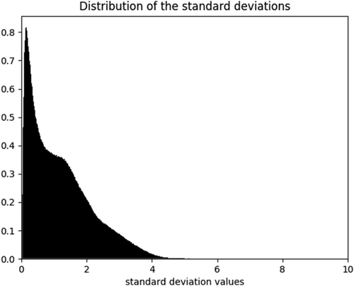
The histogram of standard deviations of the coordinate components in the CND lookup table for 5-residue segment case. The distribution peaks at a very small value of standard deviation indicating that the coordinate components of the 1st and 5th mainchain C (carbonyl) are clustered in a narrow distribution, that is, the configurational distributions of the 5-residue peptide segments are narrow. In addition, the average value of the standard deviation is 1.20 Å.
It needs to be mentioned that, in the implementation of OPUS-CSF, we assume that the smaller the CSF score, the more likely the structure to be native. This is an approximation because even a native structure may not usually have a zero CSF score. However, the narrow distributions of standard deviations of the coordinate components of mainchain C (carbonyl) atoms (Fig. 1) suggests small scores for the native structures. Figure 2 shows a population distribution of the CSF scores for 278 native structures in 11 decoy sets (per independent coordinate component). The average value of the native CSF scores is 0.84 and the standard deviation is 0.27. Thus, in native structures, the deviations of the coordinate components from their average values are less than one standard deviation of the coordinate component distribution in CND lookup table. The fluctuation of the native CSF scores is also very small.
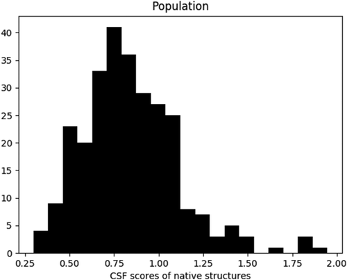
The population distribution of CSF scores for 278 native structures in 11 decoy sets. The X-axis is the CSF score (per independent coordinate component variable). The Y-axis is the histogram of the population.
Figure 3 shows the frequencies of sequence repeating in the CND lookup table in 5-residue case. In principle, the more times a sequence repeats in PDB, the better statistics one would have for that sequence in CND lookup table. In the 5-residue case, half of the sequences repeat >26 times in the distribution. The largest value of X-axis is 29,618 with one sequence. In constructing CND lookup table, there is always an issue between the sequence diversity and sequence repeating frequency in PDB.
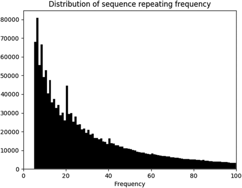
The distribution of frequency of sequence repeating in the CND lookup table. The X-axis is the repeating frequency, and the Y-axis is the number of sequences with particular repeating frequency. Sequences that repeat less than five times were omitted in our study. Analysis of this distribution indicates that half of the sequences repeat >26 times. The largest value of X-axis is 29,618 with one sequence, but not shown for the purpose of clarity.
We examined OPUS-CSF using different length of segments. As the length of segment increases, naturally the coverage decreases, and the ratio of the number of segments that appear more than five times to the total number of segments in PDB decreases (Table 3). On the other hand, if Coverage is defined as the ratio between the number of segments available in CND lookup table and the number of total segments of a test sequence, the average coverage of the 11 decoy sets (in total 278 targets) decreases as the length of segment increases. If a test sequence has <20% of its segments available in the CND lookup table, that is, its coverage is <20%, it is regarded as Unknown, then the number of unknowns increase as the lengths of segments increase. More details of OPUS-CSF on different segment lengths can be found in Supplemental Information.
| Num_above5 | Num_all | Num_above5/Num_all | |
|---|---|---|---|
| 5-residues | 1766273 | 2350969 | 0.751 |
| 7-residues | 3736778 | 9544858 | 0.391 |
| 9-residues | 3713506 | 10262243 | 0.362 |
| 11-residues | 3743204 | 10698802 | 0.350 |
- a Num_above5 is the number of sequence segments which occur at least five times in PDB. Num_all shows the total number of sequence segments in PDB. The ratio decreases as the length of segments increases.
The 5-residue case delivers the best performance in terms of decoy recognition (244 out 278 native recognition in Table 4). However, the Z-scores are better for longer-segment cases. This is probably because the longer segments preserve more sequence homology information.
| 5-residues | 7-residues | 9-residues | 11-residues | |
|---|---|---|---|---|
| Success numbers | 244 (278) | 218 (278) | 220 (278) | 219 (278) |
| Z-scores | −3.56 | −4.55 | −4.62 | −4.57 |
| Average Coverage | 0.971 | 0.749 | 0.712 | 0.683 |
| Unknowns | 0 | 41 | 45 | 46 |
- a Success numbers are the numbers of native structures that OPUS-CSF correctly recognized from the decoys. Numbers in parentheses (278) are the total number of native structures (or targets) in 11 decoy sets. The Z-scores are the calculated for the CSF scores of the native structures with respect to their decoys. Coverage means the ratio between the number of segments available in CND lookup table and the number of total segments of a target sequence. The table shows the average coverage among 278 targets in 11 decoy sets. Unknowns are the numbers of target sequences that have <20% of coverage. For these sequences, OPUS-CSF is not applicable. Note, 5-residue case does not have sequence classified as unknown, while 7-residue case, for example, has 41 out of 278 sequences not applicable for OPUS-CSF. The number of unknown increases slightly as the length of segment increases. Note, in the combined segment case, the longer segments may make no contribution to the CSF score if they are unknowns. Since the 5-residue segment case has no unknowns, it guarantees OPUS-CSF applicable to all target sequences even in rare ones that all longer segments are regarded as unknown.
For the 5-residue case, we also tested a scenario by constructing CND lookup table using four residues (1, 2, 4, and 5), instead of using two terminal residues (1, 5). The number of native recognition and Z-score are 226 and −3.60, while, in the case of (1, 5), they are 244 and −3.56 (as indicated in Table 4). This is very interesting as it indicates that using two terminal residues (1, 5) captures a better coarse graining level than using more residues (1, 2, 4, and 5).
OPUS-CSF has some obvious advantages. First, the CND lookup table is constructed directly from the entire PDB, and it contains the information of all allowed configurational information of the native segments (at least for the ones repeated more than five times in PDB). The results seem to indicate that it is better than Boltzmann formula based methods. Second, the speed of OPUS-CSF is very fast, especially for longer polypeptide chains. This is because the entire chain is scanned once and linearly, it only requires partial mainchain atom coordinates to calculate the CSF score for a structure. Unlike other potentials such as GOAP40 and OPUS-PSP,34 no inter-atomic distances need to be calculated. We want to emphasize that, in modeling protein structures, an empirical potential function or a scoring function, should be fast and accurate. In early stage of modeling, it is advantageous that the scoring function requires minimal amount of structural information. In this regard, OPUS-CSF seems to be a good choice.
Methods
Scanning through the polypeptide chain with a step size of one residue, we collected small peptide segments with sequence length of 5, 7, 9, and 11 residues and searched for their configurations in the entire PDB. Totally, we downloaded 130,054 PDB structures on June 7, 2017 via ftp://ftp.wwpdb.org/pub/pdb/data/structures/divided/pdb. The sequences that appeared less than five times in PDB were discarded. The number five was chosen empirically. Peptide segments with poorly resolved structures such as broken bonds were not included.
Here we use 5-residue segment case as an example to illustrate the details of the procedure. The ratio of segments that appear more than five times to all segments in PDB is 75.1%, which means we can utilize 75.1% of the information in the whole PDB using 5-residue segments (also see Table 3 in Results and Discussion).
A local molecular coordinate system was defined for every segment using the positions of three main-chain atoms in the middle residue. The origin was set at the Cα atom, the X-axis was defined along the line connecting Cα and C (carbonyl) atoms, Y-axis was in the Cα -C-O plane, parallel to component of C-O vector that was perpendicular to the X-axis, and the Z-axis was defined correspondingly (Fig. 4).
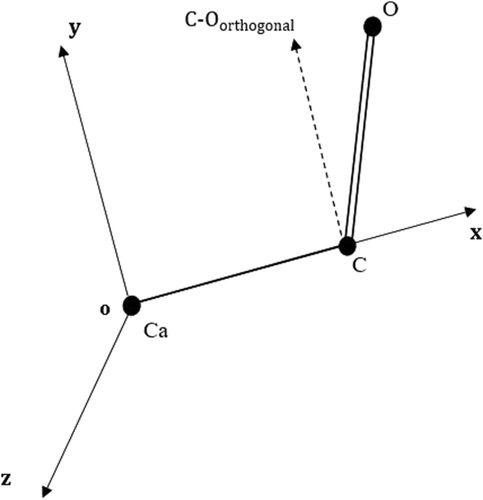
Local molecular coordinate system in OPUS-CSF defined by the mainchain atoms of the 3rd residues. The origin is on Cα atom. The X-axis is along the Cα–C line. Y-axis is in the plan of Cα–C–O atoms, and parallel to the orthogonal projection of C–O vector. Z-axis is defined accordingly.
For a 5-residue segment with a specific sequence, we saved the mainchain C (carbonyl) coordinates of the 1st and 5th residue in the local coordinate system, denoted as
 and
and
 . And under our assumption, we treated coordinate components
 as six independent variables. By scanning through the entire PDB, we generated six independent distributions of these variables, called configurational native distributions (CNDs) of 5-residue segments. We then calculated the means and standard deviations of the distributions and they were kept as the CND lookup table.
For a test structure, we scanned through its sequence with 5-residue-segments. For each segment and its sequence, we looked for the Z-scores of the six independent variables in the CND lookup table. At the end, we added up all the absolute values of Z-scores of all variables for all segments, and it was called CSF score. We assume the structure with smallest CSF score has the largest likelihood to be the native structure.
The segments of varying lengths are denoted as 5(1, 3, 5), 7(2, 4, 6), 9(1, 3, 5, 7, 9) and 11(2, 4, 6, 8, 10). Here, in segments with the form of 5(1, 3, 5), for example, the first number 5 is the segment length, 1,5 in the parenthesis are the residues that we record C (carbonyl) atom positional distributions in local coordinate system, 3 is the residue on which the local coordinate system is defined. For 9(1, 3, 5, 7, 9) and 11(2, 4, 6, 8, 10), four atoms are used for recording mainchain C (carbonyl) positional distributions, thus totally 12 independent variables are used.
The CSF score can be calculated either based on one particular segment length or by combining all segment length together. In the case of combined segment length, final CSF score is a linear sum of all CSF scores of different segment length. No weighting function is introduced for the contribution of different segment lengths.
The 11 commonly used decoy sets we used to test OPUS-CSF are the same as those used in GOAP,40 including decoy sets of 4state_reduced,59 fisa,58 fisa_casp3.58 hg_structal, ig_structal and ig_structal_hires (R. Samudrala, E. Huang, and M. Levitt, unpublished). I-TASSER,39 lattice_ssfit,60, 61 lmds,62 MOULDER63 and ROSETTA.64
Accessibility of OPUS-CSF
The scoring function is freely available to the academic community.
Acknowledgments
The authors wish to thank Robert L. Jernigan for careful reading of the manuscript and numerous comments on how to improve it. J.M. thanks support from the National Institutes of Health (R01-GM067801, R01-GM116280), and the Welch Foundation (Q-1512). Q.W. thanks support from the National Institutes of Health (R01-AI067839, R01-GM116280), the Gillson-Longenbaugh Foundation, and The Welch Foundation (Q-1826).


