A density-based time-series data analysis methodology for shadow detection in rooftop photovoltaic systems
Funding information: Rijksdienst voor Ondernemend Nederland; Netherlands Enterprise Agency (RVO), Grant/Award Number: TEUE117067
Abstract
The majority of photovoltaic (PV) systems in the Netherlands are small scale, installed on rooftops, where the lack of onsite global tilted irradiance (GTI) measurements and the frequent presence of shadow due to objects in the close vicinity oppose challenge in their monitoring process. In this study, a new algorithmic tool is introduced that creates a reference data-set through the combination of data-sets of the unshaded PV systems in the surrounding area. It subsequently compares the created reference data-set with the one of the PV system of interest, detects any energy loss and clusters the distinctive loss due to shadow, created by the surrounding objects. The new algorithm is applied successfully to a number of different cases of shaded PV systems. Finally, suggestions on the unsupervised use of the algorithm by any monitoring platform are discussed, along with its limitations algorithm and suggestions for further research.
1 INTRODUCTION
1.1 Motivation
The worldwide photovoltaic (PV) installed capacity has grown exponentially the past years, from 25 GW in 2008 to at least 942 GW at the end of 2021.1, 2 In May 2022, the 1 TW milestone has been reached.3 Similar growth is observed in the Netherlands: The national PV installed capacity has increased from 59 MW in 2011 to 6.9 GW in 2019,4 10.7 GW in 2020,5 and 14.4 GW by the end of 2021.6 At the end of 2016, 70% of the installed capacity was attributed to small-scale residential installations on rooftops.7 In the past years, this number is declining, since new small scale installations are constantly below 50% of the annual installed capacity, although it remains at high values, 49% in 2017,8 38% in 2018,9 35% in 2019,4 31.4% in 2020,5 and 35.2% in 2021.5 Thus, small-scale residential installations still form a large share of the total installed capacity in the Netherlands. While their share in the market is decreasing, the number of PV systems on rooftops is expected to keep increasing. Furthermore, the European Commission has been promoting the increase of residential PV systems since 2010 through the Energy Performance of Buildings Directive (EPBD) that provides guidelines with the aim of the realisation of net zero-energy buildings.10
The complexity of the urban environment imposes a challenge for the application of PV systems on rooftops, where different objects, (i.e., poles, chimneys, dormers, and nearby trees and buildings) can obstruct the solar irradiance, which will decrease the energy output of the installed solar panels.11 As a result, PV systems installed in urban environments are under-performing, especially compared with the ones installed in rural environments, and their performance is (further) reduced in areas with higher building density and higher average building height.12
Monitoring of residential small-scale PV systems faces four main challenges: first, the lack of onsite global tilted irradiance (GTI) due the relatively high cost of a pyranometer; second, the presence of shadows that affect the monitored panels but not any chosen reference data, either local (pyranometer, neighbouring PV systems) or not (satellite, local weather station); third, in residential systems, power measurements are obtained through the inverters or low cost data-loggers with lower accuracy and smaller resolution, compared with large-scale PV plants; finally, in a residential environment with different buildings and rooftop areas, tilts and orientations of PV systems may vary. Monitoring of large numbers of PV systems with diverse characteristics requires complex and costly data inspection; thus, an unsupervised performance monitoring system that includes automated malfunction detection is preferred.
In this paper, a new shadow detection algorithm is introduced that tackles the challenges mentioned above by creating a reference data-set for any studied PV system, detecting the moments that the system is malfunctioning and distinguishes the shadow from other malfunctions.
1.2 Literature review
This paper focuses on the automatic malfunction detection of PV systems and focuses on the identification, within the detected malfunctions, of any shadows that occur due to objects in the close vicinity. The first guideline on malfunction detection of PV systems is based on the widely known Performance ratio, introduced in 1998.13
In the past 25 years, the evolution of data science in combination with the increase of computing capacity led to more sophisticated and precise malfunction detection and shadow identification methods. The performance ratio is simply calculated by dividing the total produced energy with the total reference one.
Later in the 2000s, it was combined with malfunction patterns.14, 15 In the same period, the simulation of PV production from solar irradiance and other weather conditions was introduced.16
After 2010, more methods based on the comparison with simulated power or voltage have been successfully introduced,17-20 along with more PV performance simulation models21 and a method that was able to determine the location of the fault22 in a PV plant. Furthermore, the impact of shadow along with maximum power point tracking (MPPT) control was proposed.23
In 2015, in the framework of IEA-PVPS (International Energy Agency - Photovoltaic Power Systems Program) TASK 13,24 a report with scatter-plots of different characteristic malfunctions was introduced.25 The collection of plots (named “stamp collection”) was assisting the user to the identification of malfunctions on PV systems through visual inspection. In this “stamp collection,” many cases of shading were included among the “stamps.” In the same year, Sinapis et al26 studied the effect of the identical shading on three PV systems with the same panels but different system designs (string inverter, power optimisers, and string inverters). Based on the same system, a simulation model was developed to quantify the benefits and drawbacks of different PV system architectures.27
Later, in 2016, two newly introduced fault detection algorithms allowed to detect different types of faults, with shadow among them, one on the DC part28 and one by comparing the I-V curve at normal operation and the I-V curve at shading conditions.29 Furthermore, a method based on a different philosophy was proposed, able to predict faults due to shadows (and other technical faults).30
In 2017, several methods were introduced for automatic fault and shadow detection. Malor et al. monitored identical sets (sister arrays) connected to the same inverter of the PV system.31 Topic et al. introduced a model for detecting an optimal PV system configuration for a given installation site,32 where the effect of the inter-row shading is modelled. A different approach of shading detection, since it is taking place on the direct current (DC) side, was proposed in Garoudja et al.33
In 2018, the “real PR” method that will be used later in this paper was introduced.34 Another, different approach for shadow identification is presented in Bognár et al,35 where PV system and weather data are processed by the support vector machine (SVM). LIDAR (light detection and ranging of laser imaging detection and ranging) has been used as well in a LiDAR-based model for shadow identification36 with quite promising results.
From 2019 onwards, several malfunction detection methods have been introduced. A monitoring tool that combines thermography and artificial inteligence for fault detection and filtering of non-significant anomalies was introduced by Haque et al.37 Another approach, based on analysing high-frequency components of voltage signals derived from Kalman filters, is presented in Ahmadi et al,38 to detect series of arc fault occurrences. An unsupervised and scalable framework for fault detection in time series data was introduced in Pereira and Silveira.39 Alternatively, Harru et al. focused on the DC side of PV systems and the detection of temporary shading with the use of a model based on the one-diode model and a one-class support vector machine (1SVM) procedure.40 Moreover, drones were successfully used for temperature monitoring of PV plants on large rooftops.41
More recently, in 2020, Karimi et al. focused on hot spot detection with the use of a Teager-Kaiser energy operator technique and a hot spot detection index.42 An interesting approach for PV output energy modelling by combining a new data filtering procedure and a fast machine learning algorithm named light gradient boosting machine (LightGBM) was introduced in Ascencio-Vásquez et al43 and can also be used for malfunction detection. Another fault diagnosis technique, based on independent component analysis (ICA), was proposed in Qureshi et al.44 Yet different approaches, based on malfunction forecasting, are introduced in Vergura45 and He et al.46 In the first paper, authors detect low-intensity anomalies before they become failures, while the second is based on similarities of inverter clusters of a PV system.
Finally, in 2021, several interesting papers in the field of PV systems monitoring based on data science have been published. In Murillo-Soto and Meza,47 an automated reconfiguration system is proposed to detect and manage two types of faults at any position inside the solar arrays. Similarly, in Chao and Lai,48 a malfunction/shadow detection method is introduced that triggers the reconfiguration of the array for maximum output power. Finally, a different approach is presented in Catalano et al,49 where an efficient method for photovoltaic arrays study through infrared scanning (EMPHASIS) is proposed for malfunction detection and power estimation at cell level, with excellent results.
1.3 Paper organisation
The remaining part of the paper is organised as follows: In Section 2, the scope of the new algorithm is discussed, with its limitations, and the necessary data preparation and description of the commercial PV systems where the algorithm is tested. Section 3 is concerned with the methodology used for this study, describes the five different steps of the introduced algorithm in Sections 3.1 to 3.5, and verifies it in Section 4. In Section 5, the new and the old algorithm are applied on commercial PV systems, focusing on three key themes.
In Section 5.2.3, the new algorithm is applied unsupervised to different cases of shaded PV systems for specific years of data. In Section 5.1, it is applied to MLPE systems with different shadow patterns, while in 5.2, it is applied to a PV system with string inverter. In the final part of Section 5, Section 5.2.1, some interesting and distinctive examples of shadow and shadow detection are presented.
In Section 6, the effectiveness and the limitations of new algorithm are discussed and suggestions for further research are presented, while in Section 7, the conclusions of this study are presented.
2 SCOPE AND DATA OF THE NEW ALGORITHM
2.1 Scope of the introduced algorithm
The purpose of this paper is the development of a monitoring algorithm that automates the analysis and monitoring of partially shaded PV systems on rooftops. The new algorithm is build based on two older algorithms, developed based on PV production data extracted using a testing facility,34, 50 and it is adjusted according to the needs of data extracted from residential systems.
The proposed method focuses on malfunctions detected by a malfunction detection algorithm, called “Real PR,”34 or “Real Performance Ratio.” The new algorithm clusters the detected malfunctions either to groups of shadows or classifies them as faults. Then, the ones clustered in groups are further studied, in order to investigate if they are resulting from shading of the same object and detect periods within groups where the shadow could not be detected due to high diffuse irradiance. Finally, it creates a profile for each shadow that affects the system.
The resulting shadow profile can be used to calculate the energy loss due to any obstacles and to predict the shadow in a future year in order to immediately distinguish it from any occurred malfunctions.
- Create reference data-set for the studied PV system
- Cluster the data to normal (inliers) and non-normal (outliers) operation with the application of the “Real PR” algorithm.
- Analyse only the outliers and detect the groups in the date vs. time scatter-plot with higher density.
- Merge the groups of the previous step, based on solar azimuth in larger clusters, that is, the shadows.
- Detect the date and time boundaries for every cluster of groups.
- Characterise as shadow all the measurements within the boundaries and create the shadow profile.
The first step 0 is preparatory and involves the creation of the reference data-set, fitted to the studied PV system. Since no data science techniques are used and can be skipped if a pyranometer or reference cell exists, it is designated as step zero.
2.2 Data preparation
Two different data-sets are required for the application of the proposed algorithm, the power output (either AC or DC) of the studied PV system (referred to as “studied PV” from now on) and the reference data (referred to as “reference data” from now on).
2.2.1 Data of studied PV system
The selection of the actual unit depends on the available reference data. If the reference data are solar irradiance or power of a differently sized PV system, then system yield is selected. Power could be used as well if a PV system with identical capacity is used as reference.
In this study, both options are used: (1) when the reference data is power of identically sized PV systems, the power output of each of the panels is used as data of the studied PV, and (2) when PV systems with string inverters are compared with panels from system with module level power electronics (MLPE), system yield ( ) is used.
2.2.2 Reference data
Reference data could vary depending on the studied PV system. In testing facilities or large PV plants, solar radiation from pyranometers or reference cells is usually available. However in residential, small-scale PV systems, mounted on rooftops, the availability of such data is a luxury. Thus, different sources should be used, such as the power output of a neighbouring PV system, with same tilt and orientation (also known as peer-to-peer (P2P) comparison).
The data selection method demands the knowledge of the system and cannot be applied automatically to a large number of PV systems already installed and with only available information on the usual static (meta-)data (tilt, orientation, capacity, location, etc.)
In this paper, PV systems with power optimisers are used; thus, each panel can be treated as an independent PV system and all the other panels as different PV systems in the same neighbourhood. Similarly, for the development of the “real PR” algorithm in Tsafarakis et al,34 and for its use in Tsafarakis et al,50 data from MLPE systems were used and for each studied shaded panel, and the average production of the unshaded panels of the system was used as reference data.
In order to create a reference data source for any panel of a random MLPE system, in this paper as reference data for a selected panel, the production data of all the other panels of the system are used. For each timestamp, the panel with the highest power output is selected, thus being the one with the lowest possibility to be shaded or malfunctioning.
2.3 Data source
The proposed method was developed by using data from 5 different PV systems mounted on rooftops in the city of Breukelen, the Netherlands (52.1710° N, 5.0013° E). The PV systems consist of identical panels, with capacity of 260 Wp per panel and identical power optimisers. The total capacity varies per system, from 2340 Wp (9 panels) to 4420 Wp (16 panels).
Tilt and orientation varies within the panels of each PV system; thus, seven different tilt and orientation combinations are forming the studied sample. Due to the power optimisers, each panel can be considered as a separate PV system; thus, the study sample consist of 69 panels-system, all with the same capacity (260 Wp) and 7 different tilt and orientation combinations. Tilt varies from 13° to 40° and orientation from 142° to 234° (South is 180°).
In all the PV systems of the sample, each MLPE device measures using different time stamps. Thus, data had to be re-sampled to at least 10 minutes time resolution in order to create samples with comparable date-time index without empty (NaN) timestamps.
Due to privacy regulations, exact locations nor photos of systems can be provided.
3 DESCRIPTION OF THE ALGORITHM
The new algorithm is divided in five steps, and each step is described and visualised in the following five subsections. Each subsection contains two or three subsections, where in the first (3.X.1) the principle of the step is explained, in the second (3.X.2) the step is applied to a shaded PV panel with power optimiser and visualised for better understanding, and in the third (3.X.3) the results are discussed. The process is summarised in a flowchart in Figure 1 for better understanding.
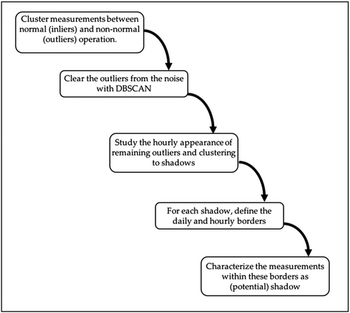
In the presented example the power of a shaded solar panel with power optimiser is used. The panel is part of a PV system mounted on a rooftop with South-West orientation (220°). From an initial exploration of the data, it was suspected that the panel was shaded by an object in the morning, which was confirmed after visual inspection using satellite imagery and Google street services and photos provided by the installer. In Figure 2, the PV system is presented with the panel of the example pointed by a green arrow. It is placed on the extension of the house together with five more panels. The panel is shaded by the main part of the house due North-East, obviously in the morning.

3.1 Step 0: Creation of reference data-set
The reference data are calculated by the new automatic method, introduced at the end of Section 2.2.2. The production data of the other five panels mounted on the extension of the house are used. For each timestamp, the output of the panel with the highest power is selected and the data are re-sampled to 10 min time resolution in order to create samples with identical date-time index, similar to the data of the studied system.
The remaining eight panels installed on the tilted rooftop have considerably different tilt (35° vs. 13°); thus, they cannot be used for the creation of the reference data-set.
3.2 Step 1: Detection of the outliers
3.2.1 Explanation
The first step of the new algorithm is to detect outliers in the analysed sample. The clustering algorithm “real PR” developed and tested by the authors in a previous study34 is applied and clusters the measurements into outliers and inliers. The inliers are following a linear relationship between the studied PV and the reference data, while the outliers are the measurements that fail to follow this relationship. These are the moments where the studied PV is failing, thus the moments where the new algorithm will search for a shadow in the following steps.
3.2.2 Application and visualisation of step 1
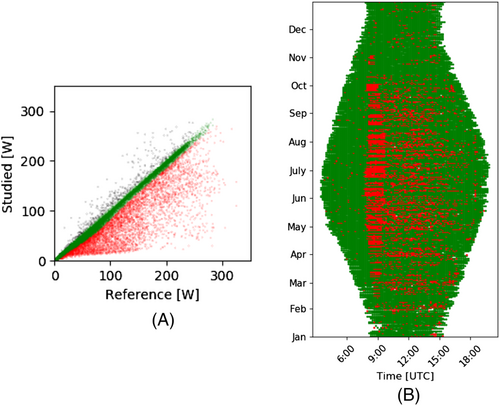
The measurements are divided in inliers and outliers by the clustering algorithm “real PR.” In Figure 3A, an example has been presented, where the green markers are the inliers and the red markers the outliers that will be further studied in the next steps. The measurements are additionally plotted in a time versus date scatter-plot and illustrated in Figure 3B. Closer inspection of the plot shows that the outliers are concentrated around specific periods (i.e., during morning hours), where their density is higher. In the next step, these periods will be grouped and distinguished from the random faults, based on the density variation.
3.3 Step 2: Clear outliers from the noise
3.3.1 Explanation
In step 1, the moments where the studied PV system is failing are detected. In step 2, their density in a time vs. date scatter-plot is studied. The non-parametric clustering algorithm “Density-Based Spatial Clustering of Applications with Noise” (DBSCAN)52 is preferred for this step due to the presence of noise in the scatter-plot (Figure 3B). Through DBSCAN, outliers in areas of higher density than the rest of the data-set are clustered into groups, named “DBSCAN groups,” which will be further studied in the following steps.
Data points in sparse areas are considered to be noise and excluded from the rest of the analysis for shadow detection. However, they will be analysed during the verification of the algorithm (Section 4) and further discussed in Section 6.
3.3.2 Application and visualisation of step 2
Figure 4 illustrates the impact of step 2 on the outliers. DBSCAN clusters high density areas into groups and characterises measurements in low density areas as noise. In Figure 4, outliers clustered in DBSCAN groups are coloured using various colours while the ones characterised as noise remain red.
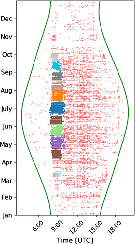
In the DBSCAN algorithm, a point is characterised as “core point” if within the area of 20 min in x-axis and 5 days in y-axis (a rectangle in the plot); 65% of the possible measurements exists that can fit, depending on the data resolution. For instance, in the presented example of 5-min data resolution, in a period of 40 min and 10 days, a maximum of 80 measurements (either inliers or outliers) could fit. Thus, a single measurement is considered as “core point” if more than 51 outliers exist within the area around it.
3.3.3 Discussion of step 2
Interestingly, the output of DBSCAN for the same shadow yields several small groups instead of a larger one. The dependence of shadow on the irradiance conditions leads to this separation, since in periods where diffuse irradiance is dominant, the creation of a shadow is limited and the density conditions of DBSCAN are not met. These periods can be seen in Figure 4, as the empty areas (sometimes with red dots) between the DBSCAN groups. Hence, groups of the same shadow should be connected in a larger one, the shadow, an action that takes place in the next step.
3.4 Step 3: Cluster remaining outliers to shadows
3.4.1 Explanation
In step 3, the frequency of outliers clustered into DBSCAN groups during the day is studied, in order to detect any connection between DBSCAN groups. A similar process has been used successfully in the previously developed method, “shadow profile,”50 directly after the initial clustering to inliers and outliers. In the new algorithm, the outliers are further processed through DBSCAN, and the majority of the noise is filtered out. Thus, step 3 is applied for the categorisation of different shadows that may exist during the day (morning–afternoon, etc.), by studying the appearance of the outliers of DBSCAN groups during the year.
3.4.2 Application and visualisation of step 3
Figure 5 illustrates the operation of step 3. The graph represents the distribution of the outliers, clustered in DBSCAN groups in step 2, during the day. Between 7:45 and 10:00 (UTC timezone), the frequency of outliers is higher than the average. Thus, all DBSCAN groups within that moments are reordered as one unique shadow.
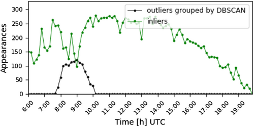
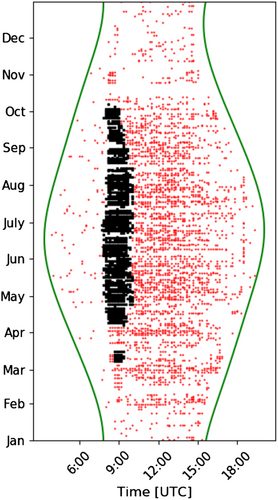
Once the DBSCAN groups are connected, based on the allocation of their outliers on time, the merged shadow clusters are formed. Figure 6 illustrates the results of step 3 after applying it to the data of Figure 4. All the small groups are merged and a larger group is formed, illustrated with black dots.
3.4.3 Discussion of step 3
The outliers of the detected shadow are coloured black in Figure 6, while the rest, the ones characterised as noise, are still coloured red. Empty areas or even some filled outliers can be seen within the shadow, especially from mid March to mid April. In these cases, the outliers do not meet the density criteria of DBSCAN in order to be clustered in a group. However, through the allocation of the DBSCAN groups, it can be assumed that it is the same shadow, although the irradiance for that period was not high enough in order to create a shadow and consequently, a visible impact on the data. In the next step, these gaps are going to be filled in order to cover the complete date-time period of the possible expected shadow.
3.5 Step 4: Define the contour of each shadow
3.5.1 Explanation
During this step, the results of the two previous ones are combined to estimate the period that the shadow of a single obstacle is expected to affect the studied PV system. The algorithm aims to detect the contour of the shadow and denotes all the included measurements, both outliers and inliers, within the contour as potential parts of the shadow.
The contour consists of four boundaries: two date-dependent ones, the first day and the last day of the shadow during the year, and two time-dependent ones, the starting and the ending times during each day. Thus, the date boundaries considered the first day and the last day of the shadow as selected from step 3.
The estimation of the time-related boundaries, left boundary for the beginning, right for the end of the shadow demands a process that depends on the solar position, which changes during the year due to Earth's orbit around the sun. Each boundary can not be represented by a single value (time), especially for a long period, but from a continuous data-set. Since the shadow is already divided into DBSCAN groups, they are used for the selection of these data-sets. For the left boundary's data-set, the earliest moments of each DBSCAN group are selected and, similarly, for the right boundary, the latest one(s). Thus, two data-sets are created, with length equal or larger than the number of DBSCAN groups. However, these moments cannot be used as boundaries since a single moment for each DBSCAN group will lead to stair curve boundaries. In order to obtain continuous ones, polynomial fits are made. These models are trained to detect the relationship between the day of the year and the solar azimuth of the data-sets. Aim of the models is to use as input the day of the year and based on the training to estimate the solar azimuth for the rest of the days that the shadow exists. The solar azimuth of each measurement is preferred instead of the timestamp, due to its higher range of values and resolution; thus, each measurement has a unique azimuth value.
3.5.2 Application and visualisation of step 4
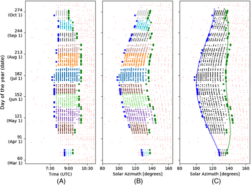
In Figure 7, step 4 is illustrated. Figure 7A,B represents the data selection for the left (blue squares) and right (green) time boundaries. In Figure 7A, the earliest and the latest moments, based on time, of each DBSCAN group are picked as training sets for the polynomial models. In Figure 7B, the same data are plotted in a date versus solar azimuth scatter-plot; these values are used as training input in the polynomial models. The trained polynomial models are using as input for all the days of the year for which shadow occurs (thus the days between the day dependent boundaries) and return the left and right boundaries of the shadow. This is shown in Figure 7C.
3.5.3 Discussion of step 4
The selection of the training set is based on time and leads to the selection of multiple points per DBSCAN group (Figure 7A), thus to a larger training set and finally to a more accurate prediction model. However, the use of solar azimuth instead of time in the training set leads to a smoother and more representative curve. This is visible in the connection of the first DBSCAN group (beginning of March) with the others, where there is a period (mid March to Mid April) for which the presence of shadow is weak and cannot be detected through DBSCAN. In several cases, similar to the presented example, the use of time, instead of azimuth, leads to straight lines in Figure 7C.
3.6 Step 5: Characterisation of the measurements within contours
3.6.1 Explanation
In the fifth and final step of the algorithm the measurements within the boundaries, calculated in step 4, are characterised as shadow. Although, a considerable number of inliers lies within these boundaries, these are considered as shadow that were not observed, due to the dependence of shadow on weather conditions, as mentioned in Section 6.1.1. However, it is expected that under conditions of higher solar irradiance, power loss would be observed at these moments.
3.6.2 Application and visualisation of step 5
In Figure 8B,C, the outcome of the algorithm is presented, along with the initial clustering, in Figure 8A, for better understanding. In Figure 8B, the boundaries of the shadow are plotted over the initial clustering, while in Figure 8C, the area within the boundaries, in between which shadow is observed and expected, is marked as black, while the rest of the year, where no shadow is detected, data are marked as green.
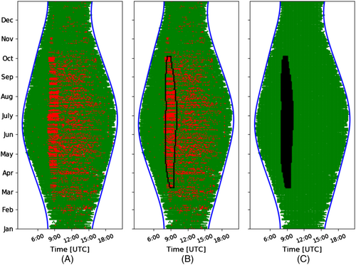
In Figure 8B, the comparison of the initial clustering with the results of the shadow detection algorithm is easier, since both are presented in the same plot. This plot format is used in the rest of the paper for the illustration of the results in Section 5.
The introduced algorithm successfully distinguishes normal and non-normal operation of the studied solar panel, as can be seen in Figure 8B,C. In the rest of the studied period, no shadow is expected by the algorithm; thus, any outliers are still characterised as measurement faults, as explained in Section 6.1.2. These are studied separately in Section 4. Moreover, from the comparison of Figure 8A,B, it can be seen that a significant number of measurements, initially characterised as inliers in Section 3.1, are finally characterised as shadow. These are the cases of shadow that “exist but cannot be observed,” as explained in Section 6.1.1 and are further studied as well in Section 4, where the algorithm is verified.
The final outcome of the algorithm is the detection of the period within which the shadow impacts the studied PV system, or solar panel, in case of this MLPE PV system. Further use of this outcome is discussed in Section 6.
4 VERIFICATION OF THE ALGORITHM
The introduced algorithm processes the outliers of a PV system and detects, based on density clustering, the ones caused by a shadow of a stable object. Its operation is summarised in Figure 8, where the initial date vs. time plot of the inliers and outliers (Figure 8A) is converted through the algorithm to Figure 8B,C.
- Measurements initially characterised as outliers and later as shadow—red dots within the black contour in Figure 8B, or red dots in Figure 8A that switch to black in Figure 8C, referred as shadow from now on.
- Measurements initially characterised as outliers, that are remarked as inliers by application of the algorithm—red in Figure 8A, and green in Figure 8C—referred as faults from now on.
- Measurements initially characterised as inliers, that are remarked as shadow—from green in Figure 8A to black in Figure 8C—referred as “expected shadow” from now on.
The first category is the result of the algorithm and reflects its main function. The other two categories are not explained in the initial description and are further analysed in the following.
4.1 Faults: outliers not categorised as shadow
These measurements are characterised as faults due to the observed power loss, and their appearance frequency does not fit in the pattern of a shadow, as established by the new algorithm in Section 3.5. As described in Section 6.1.2, the majority of them could be measurement faults, either due to the low quality measuring equipment or due to the different timestamps occurring in the measurements in the different power optimisers.
For the study of the faults, a probability density function (PDF), estimated using Kernel density estimation,53, 54 is used. The PDF is a statistical expression that defines a probability distribution (the likelihood of an outcome) for a discrete random variable as opposed to a continuous random variable.55
In Figure 9A, two PDFs are compared of the outliers as a function of solar azimuth, which is a continuous random variable with values from 50° to 350°. The blue curve represents the PDF corresponding to the shaded panel, which is compared with the average PDF profile of an unshaded panel with similar tilt and orientation (green curve). The average PDF profile is calculated by averaging the PDFs of 13 unshaded panels from different PV systems (with similar tilt and orientation) neighbouring to the studied one. It is clear that the PDF of the shaded panel has a global maximum around 100°–140°, thus within the solar azimuth interval where the algorithm detected the shadow (Figure 7). On the other hand, the average PDF of the unshaded panels for the same solar azimuth interval is a smooth curve, with a global maximum between solar azimuth 200° and 220°, where the studied panel has a local maximum at 220°.
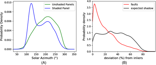
The outliers at higher solar azimuths are similar for unshaded and shaded panels. On the other hand, for the shaded panel, a local maximum is found at a solar azimuth of about 125° , which is not found for the unshaded panels.
In Figure 9B, the PDFs of the deviations of the measurements characterised as shadows and faults of the 14 panels are compared. The majority of the faults do not deviate substantially from the minimum inlier limit compared to the measurements that correspond to shadows, since the maximum of their PDF (red curve) is close to 5% deviation from the minimum inlier limit. Thus, if the “real PR” would be applied by the user with less strict parameters, these measurements could be inliers. On the other hand, the allocation of the shadows (black curve in Figure 9B) is visible in a wider deviation range, from 5% to 60%, from where it is slowly decreasing to almost zero probability around the deviation of 80%.
4.2 Expected shadow: inliers categorised as shadow
In these measurements, no power loss is observed and initially (step 3.1); these are characterised as inliers. However, they will be categorised as shadow in the final step (3.5), since they are located within the shadow barriers. As explained in Section 6.1.1, these could be cases where direct solar irradiance is a small percentage of the total tilted irradiance and shadow cannot be observed from an object. Thus, they can be denoted as “a potential shadow that cannot be seen.”
In this section. these measurements are analysed further, and results are summarised in Figure 10. For the analysis, the irradiance data from the meteorological station of the testing facility of Utrecht University is used56 as well as satellite data provided by the Netherlands Royal Meteorological Institute (KNMI).57 The outdoor test facility is equipped among others with a pyranometer for the measurement of global horizontal irradiance (GHI) and a pyrheliometer for the measurement of direct normal irradiation (DNI). The testing facility is located at the university campus, approximately 14 km from the studied PV systems.
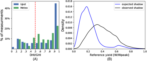
In the histogram of Figure 10A, the ratio of diffuse to direct irradiance for these measurements is presented. In approximately 70% of the measurements, where the expected shadow is not observed, the DHI was the dominant irradiance component. Thus, it can safely be assumed that due to high diffuse irradiance any faults cannot be observed during these moments, since, in contrast with the DNI, DHI is largely unobstructed by the shade-causing objects and thus still causes energy generation.
In Figure 10B, these measurements are compared with the rest of the measurements corresponding to shadow, that is, the ones initially characterised as outliers. For the comparison, their kernel density estimate plots54, 53 are plotted by using Gaussian kernels of their normalised reference power. The reference power is selected for the comparison since higher values imply higher irradiance values, thus a higher chance that shadow would be observed in a measurement and vice versa. Normalised power is used in order to provide a better reference of the level of power production.
As expected, the majority of the shadow with observed power loss is concentrated at higher reference power values, while the measurements that represent the expected but cannot be seen shadow at lower ones. Thus, it can safely be assumed these measurements are initially characterised as inliers simply due to the absence of sufficient irradiance.
5 RESULTS
In this section, the introduced shadow detection algorithm is applied to a larger sample of PV systems, and its effectiveness is tested for different cases of shadow. In Section 5.1, it is applied on three panels of different MLPE systems with different shade characteristics, while in Section 5.2, the algorithm is applied to two PV systems connected with string inverters.
5.1 Shadow detection in MLPE systems
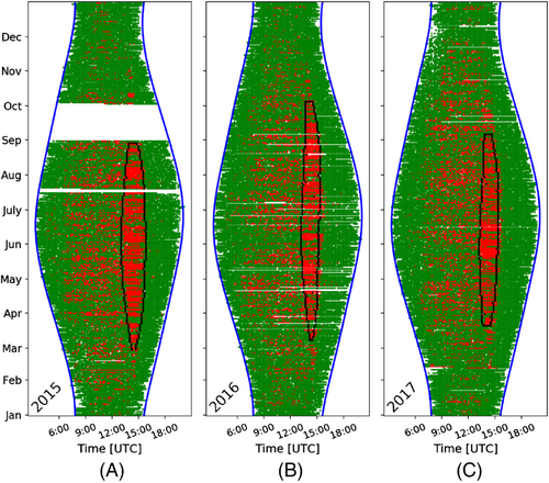
In Section 3.5.2, Figure 8, the new algorithm is applied on annual power production data of a solar panel in an MLPE PV system. In Figure 11, the algorithm is applied to the data of the same panel for all the years of the studied period. Thus, Figures 8B and 11A are the same and represent the operation of the studied solar panel during 2015, while Figure 11B,C corresponds to the years 2016 and 2017, respectively.
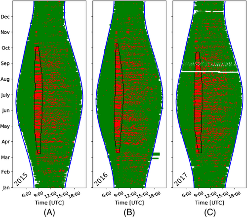
The detected shadow is created by a pole during morning hours. Minor differences are observed in its shape through the years, mostly at the ending times, while the starting and ending days are almost the same. Furthermore, the shadow starts almost the same time during the year, while the ending time differs, a fact that makes the shadow to last longer during the summer period.
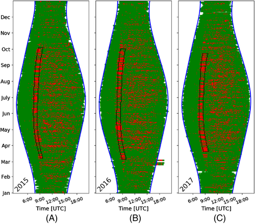
In this section, two more cases of shaded solar panels, connected to a power optimiser, are presented. The algorithm is applied to a panel that is shaded in the morning (Figure 12) and one shaded in the afternoon (Figure 13). This morning shadow, Figure 12, differs from the previous one, Figure 11, since its starting and ending times vary during the year although its duration is almost constant. These facts leads to a completely different shape of the predicted shadow that is thin and looks like a bow. However, these examples show that the algorithm is able to detect shadows with different patterns on duration and starting/ending time.
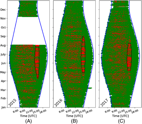
The last case in this section is of a panel that is shaded in the afternoon, see Figure 13. Both starting and ending times of the shadow as well as its duration vary during the year. Furthermore, some missing data, from August 2015 to October 2015 (subplot a), does not seem to affect the effectiveness of the algorithm and the shape of the predicted shadow is similar to the other two years, that have full data.
5.2 Shadow detection in systems with string inverters
In this example the introduced algorithm for shadow detection is applied on a PV system that is connected to a string inverter. As reference power the combination of panels of a neighbouring PV system with MLPE is used.
Similarly to the analyses of the cases with MLPE systems (Figures 11, 12, and 13), the shadow is successfully detected by the algorithm. However, small differences in the ending dates are observed between the plots. The longest period is observed in 2016, Figure 14B. On the other hand, due to the missing data during 2015, Figure 14A, the end of the shadow is detected earlier. Moreover, in late 2017 (Figure 14C), the concentration of outliers in September is lower compared with 2016, and it does not meet the spatial requirements of DBSCAN, even if higher than usual concentration of outliers can be observed by the user. This is further analysed in Section 6, where suggestions for further study and use of the algorithm are discussed.
5.2.1 More shadow examples
In this section, the new shadow detection algorithm is applied to two different cases of MLPE connected panels. In Section 5.2.2, it is applied to a shaded panel that showed a defect and was replaced during the studied period, while in Section 5.2.3, it is applied to two different MLPE connected panels on the same rooftop that are installed next to each other.
5.2.2 Shadow detection on a malfunctioning panel
This studied panel is shaded in the morning and its shadow is recognised successfully by the algorithm. Apart from the shadow, It was operating normally until July 2016, from which time it suffered from a defecting fuse and it was replaced in October 2016. The new panel operated normally during the last year of the available data, on 2017. Similarly to the previous examples, the “real PR” and the new shadow detection are applied to each year independently, and the results are presented in Figure 15.
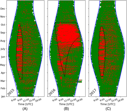
It can be seen in Figure 15A,C that the shadow has a similar pattern, which stems from similar results from the algorithm. Furthermore, in 2016 (Figure 15B), until the failure the pattern is similar with the other two years as well. However, the results of the algorithm is not following the same pattern, since it is disoriented from the large increase of the outliers after the fault occurred in July 2016.
The application of the algorithm on the detection of similar malfunctions depends on the user. An approach suggested by the authors is the following: After the first year (in this case 2015, Figure 15A), the pattern of the shadow is known. Thus, during the second year and until July, the power loss due to the shadow is expected, and no alarm is triggered. However, due to the fault, from the first occurrence of a large deviation of the expected pattern, an alarm could be triggered immediately, revealing that the extra power loss is not a shadow but a malfunction of the panel.
5.2.3 Shadow variation on back to back panels
In this example, the shadow patterns of two panels placed next to each other and shaded by the same object are studied. The distance between the panels may be limited; however, as can be seen in Figure 16, the daily duration of the shadow on one panel is almost double for the other panel. Shadows have almost the same starting time, but significantly different ending times. Starting and ending dates are the same for both shadows.
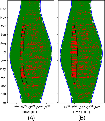
In this example, the introduced algorithm identifies successfully the shadows in both PV systems and serves as perfect example of how important the positioning of the panels is on the rooftop relative to an shading object and the difference that some centimetres can make on the power production.
6 LIMITATIONS AND FURTHER SUGGESTIONS
6.1 Limitations
6.1.1 Dependence of shadow on irradiance conditions
The aim of the algorithm is the detection of any shadow created by obstacles that may be on rooftops (e.g., dormers and exhaust pipes). These obstacles are constantly present, yet their shadow is not constant, since it is strongly dependent on the ratio of the direct normal and diffuse horizontal irradiance (DNI and DHI, respectively) to the global horizontal irradiance (GHI). The higher the DNI to GHI ratio, the higher the effect of the shadow. Furthermore, the higher the DHI to GHI ratio, the lower the shade impact of an obstacle.50 Thus, within two days with different weather, large differences can be observed in the effect of an obstacle to a system, even in situations with the same solar position.50
6.1.2 Outliers outside shadow (faults)
A significant number of outliers are observed outside of the detected shadow in every example; see, for example, Figures 15 and 16. A number of factors play a role on this; however, the two major ones are not due to malfunctions but due to the components and the nature of the residential systems.
While in testing facilities or large solar parks very high accuracy devices are measuring directly the power, in residential systems, power measurements are obtained by the multiplication of the voltage and current measurements of the optimisers. The measurements obtained from these devices are considerably less accurate than the sophisticated and expensive device of the testing facility.
Additionally, the time resolution of the measurements results in a mismatch of timings of faults between the systems. In more expensive installations, like a facility, a sophisticated monitoring system measures the power at 1 s resolution, which can be re-sampled to lower time resolution, depending on the needs of the analysis. On the other hand, the time resolution in the residential systems is not constant and varies between 5 to 7 min, in the same MLPE device. Furthermore, the moment of the measurement of each MLPE device (power optimiser in this case) is not synchronised with the others of the same system. Thus, one panel could be measured at XX:12, the other at XX:15 and so forth. On a non-clear sky day, these time difference could lead to differences in power.
6.2 Suggestions for application of the algorithm
In section 3.4 of our previous paper,34 a method to estimate the power loss of the detected outliers was presented. In that paper, all the detected outliers are considered for the calculation. However, after the application of the presented algorithm in this paper, outliers due to shadow can now be isolated from the rest of the sample. The power loss due to the shadow (and thus, due to the object that is causing it) can be estimated and provided to the owner of the system, where she/he can take further action, if possible. Another key thing to remember is the dependence of the shadow on irradiance conditions, as explained in Section 6.1.1. Thus, a dataset larger than 2 years can provide a more accurate estimation about the power loss due to a shadow.
Furthermore, by processing one full year of data with the proposed algorithm, the energy losses due to a potential shadow for future years can be estimated. Thus, any new observed power loss can be identified immediately and proper actions can be taken by the operator/owner of the system for very fast repairs.
6.3 Suggestions for further studies
In a detailed observation of the shadow plots, it can be seen that some small parts of the shadow before the first day and after the last one are not detected by the algorithm. For instance, in Figure 14, before the first day and after the last day of the detected shadow, the density of red marked data points is higher than normal but only for a couple of hours per day for three to four more days. Since during the winter where the duration of the shadow is significantly shorter, the density of the red marked data points does not fulfil the requirements of DBSCAN, set in step 2, Section 3.2. In order to achieve even more detailed shadow detection, a further, local density search could be implemented by the algorithm, similar to the local search taking place in the fourth step of the original shadow detection algorithm, see Tsafarakis et al.50
A further study could be implemented in a case where two shadows exist during the day, for instance, during the morning and during the afternoon. Unfortunately, within the 60+ panels of the studied MLPE PV systems, none was shaded twice in a day, a logical fact, since a double shading fact would be highly inefficient and less productive.
7 CONCLUSION AND OUTLOOK
In conclusion, this paper describes the development of a new shadow detection algorithm and its application for the monitoring on partially shaded residential PV systems. Since the power output is the most common timeseries data for a PV system, it is the only one that is used.
The proposed algorithm creates a reference data-set, based on the neighbouring PV systems with similar characteristics. With the use of an older method, the measurements are clustered into normal and non-normal operation or faults, and colour-coded to represent them.
Then the new algorithm studies the outliers, firstly by removing the noise with the use of DBSCAN, then finds whether the outliers are occurring in the same time periods for consecutive days, followed by clustering them in the same shadow and finally defines a contour, where all the measurements within it are shadows from the same object.
The outliers outside of the contour are verified as measuring faults in our study, while the existence of an unseen shadow is verified to be correlated with high DHI/GHI ratios.
In this study a combination of the power of the surrounding solar panels is used for the creation of the reference data-set, where for each timestamp the power of the best performing panel is selected. The method is proven to be highly adequate in the presented examples and can be used as well in an online cloud-based monitoring platform, where the combined power data of neighbouring PV systems, in which panels are connected as strings to inverters, could form reference data for each monitored PV system.
The clustering algorithm DBSCAN proved very effective for the removal of noise. Since noise is very common when solar panels are monitored through satellite measurements or pyranometers that measure global horizontal irradiance, it is suggested for further use.
The algorithm delivers a contour in time versus date plots, which reflects the detected shadow. Due to variations in diffuse irradiance per year, the contour differs slightly (less than 4%) every year. Adding several years in one scatter-plot, for more accurate detection was not efficient, since DBSCAN was detecting all the noise successfully. However, when more years are available, comparison of contours may be useful for the study of progress and changes of the shadow (in case it is a tree that grows or anything that can change).
ACKNOWLEDGEMENTS
The authors gratefully acknowledge fruitful discussions with Kostas Sinapis (TNO) and Lex Schiebaan (Sundata) and Guido van Sark for providing the 3D system representation shown in Figure 2. This work is partly financially supported by the Netherlands Enterprise Agency (RVO) within the framework of the Dutch Topsector Energy (project Intelligent Health Assessment of PV Systems, IHAPS, grant number TEUE117067).
CONFLICT OF INTEREST
The authors declare no conflicts of interest.
Open Research
DATA AVAILABILITY STATEMENT
The data that support the findings of this study are available on request from the corresponding author. The data are not publicly available due to privacy or ethical restrictions.


