Flow directions of stream-groundwater exchange in a headwater catchment during the hydrologic year
Abstract
Understanding near-stream groundwater dynamics and flow directions is important for predicting hillslope-stream connectivity, streamflow generation, and hydrologic controls of streamwater quality. To determine the drivers of groundwater flow in the stream corridor (i.e., the stream channel and the adjacent groundwater in footslopes and riparian areas), we observed the water levels of 36 wells and 7 piezometers along a headwater stream section over a period of 18 months. Groundwater dynamics during events were controlled by the initial position of the groundwater table relative to the subsurface structure. The near-stream groundwater table displayed a fast and pronounced response to precipitation events when lying in fractured bedrock with low storage capacity, and responded less frequently and in a less pronounced way when lying in upper layers with high storage capacity. Precipitation depth, intensity, regolith thickness above the fractured bedrock, and proximity to and elevation above the stream channel also had an effect on the groundwater dynamics, which varied with hydrologic conditions. Our high-frequency and spatially dense measurements highlight the competing influence of groundwater inflow from upslope locations, streamwater level and bedrock properties on the spatiotemporal dynamics of flowpaths in the stream corridor. Near-stream groundwater pointed uniformly towards the stream channel when the stream corridor was hydrologically connected to upslope groundwater. However, local interruptions of the water inflow from upslope locations caused flow reversals towards the footslopes. The direction of near-stream groundwater followed the local fractured bedrock topography during dry hydrologic conditions on a few occasions after events. The outcomes of this research contribute to a better understanding of the drivers controlling spatiotemporal changes in near-stream groundwater dynamics and flow directions in multiple wetness states of the stream corridor.
1 INTRODUCTION
Near-stream groundwater dynamics and flow direction drive flowpaths between the stream channel, adjacent riparian areas, and footslopes. Stream channels cannot be considered isolated pipes (Bencala et al., 2011) and their exchange of water with fluvial deposits and floodplains makes them part of a stream-groundwater continuum known as the stream corridor (National Research Council, 2002). The continuous exchange of water, nutrients, and organic matter between surface water and groundwater is a key environmental process controlling faunal activity (Boulton et al., 1998) and nutrient cycling (Pinay et al., 1993), and attenuates point-source contaminants (Moser et al., 2003). The dynamics of the near-stream groundwater involve changes in flow direction in the riparian area (Heeren et al., 2014), with potentially great effects on streamwater travel times (Wondzell & Swanson, 1996) and nutrient removal (Zarnetske et al., 2015). Despite the acknowledged role of the near-stream groundwater in hydrological and biogeochemical processes in the stream corridor, current understanding of the mechanisms controlling water exchange between the stream channel and near-stream groundwater is incomplete (Ward & Packman, 2019).
Studies on near-stream and hillslope groundwater have evaluated the spatial and temporal relation between precipitation events and the response of groundwater and streamflow to decipher areas contributing to streamflow and to detect hydrological connectivity between hillslopes and streams (Beiter et al., 2020; Detty & McGuire, 2010b; Ocampo et al., 2006; Rinderer et al., 2017). Haught and Van Meerveld (2011) reported a rise of near-stream groundwater hours before streamflow, while groundwater in the upper hillslope increased slower than streamflow and only after rather large events. Similar results have been reported for different landscapes, where near-stream groundwater responded to precipitation before streamflow (Beiter et al., 2020; Scheliga et al., 2018; van Meerveld et al., 2015). This finding has been interpreted by the authors as a contribution of near-stream groundwater to streamflow generation, while the rise of groundwater after streamflow response has been linked to a lack of hydrological connectivity between the groundwater and the stream channel.
While shallow groundwater response to precipitation has often been linked to streamflow generation (Penna et al., 2015; Rinderer et al., 2016) and hillslope-stream connectivity (Haught & Van Meerveld, 2011), relatively few studies have addressed changes in near-stream groundwater dynamics to infer the catchment response to precipitation events for various hydrologic conditions (Beiter et al., 2020; Jencso et al., 2009; Scheliga et al., 2018). In catchment and hillslope studies, hydrologic connectivity has usually been assumed to be unidirectional, from the hillslope towards the stream channel (Blume & van Meerveld, 2015). While key hillslope-processes have been explored by this approach (Detty & McGuire, 2010a; Jencso et al., 2009; Ocampo et al., 2006), it may not be fully representative of the actual flowpaths in the near-stream groundwater since a number of studies have shown streams to be in losing conditions with little contributions to streamflow generation from the hillslopes in various hydrologic conditions (Dudley-Southern & Binley, 2015; Heeren et al., 2014; Rodhe & Seibert, 2011; Vidon, 2012).
Vidon and Smith (2007) and Rodhe and Seibert (2011) found strong temporal changes in groundwater gradients with the near-stream groundwater flow pointing towards the stream during wet conditions and parallel to the stream channel during drier conditions. This behaviour cannot be generalized since near-stream groundwater has also been observed to point towards the stream before events and towards the hillslopes following discharge increase during events (Dudley-Southern & Binley, 2015; Vidon, 2012; Vidon & Hill, 2004) or to point predominantly down-valley with no substantial changes even during high-intensity storm events (Voltz et al., 2013). Van Meerveld et al. (2015) used a well network at a hillslope-riparian site and found that hillslope-stream connectivity was only active during intense precipitation events, triggering the temporal re-appearance of streamflow and sustaining groundwater levels with gradients pointing towards the stream channel. Near-stream groundwater flow direction varied most around bedrock depressions (van Meerveld et al., 2015) and during high-flow events when the groundwater table rose into different layers of the subsurface (Heeren et al., 2014). Overall, individual studies provide contrasting results, which hampers to derive a generalisable understanding of the drivers of water exchange between the stream channel and the adjacent groundwater (Ward & Packman, 2019).
Several attempts were made to decipher the effect of different drivers on groundwater dynamics and flow direction (Rinderer et al., 2016; Vidon, 2012). Hillslope studies showed that shallow groundwater response to precipitation was related to topographical location (Rinderer et al., 2016), soil depth (Penna et al., 2015), bedrock topography (Tromp-Van Meerveld & McDonnell, 2006), precipitation characteristics (Dhakal & Sullivan, 2014; Fannin et al., 2000), and antecedent conditions (Detty & McGuire, 2010a). However, compared to hillslopes, near-stream groundwater dynamics are also affected by the local accumulation of finer soil material in the riparian zones (Rinderer et al., 2017; Scheliga et al., 2018), streamwater infiltration (Dudley-Southern & Binley, 2015), and changes in gradients due to streambed morphology (e.g., pool-and-riffle sections, Buffington & Tonina, 2009). Studies investigating the near-stream and hillslope groundwater also highlighted the higher degree of variability of groundwater flow direction in the near-stream domain compared to upslope locations (Burt et al., 2002; Hinton et al., 1993; Rodhe & Seibert, 2011; Von Freyberg et al., 2014).
- How and why does the near-stream groundwater table dynamic vary in different hydrologic conditions?
- How and why does the near-stream groundwater flow direction change in different hydrologic conditions?
2 STUDY SITE
The study site is a 55 m long corridor along a headwater stream in Luxembourg (49o49'38″N, 5o47'44″E) downstream of the Weierbach experimental catchment (Hissler et al., 2021). The geology consists of Devonian slate and quartzite bedrock, covered by Pleistocene periglacial slope deposits. The climate is semi-oceanic with precipitation rather uniformly distributed throughout the year. Higher evapotranspiration rates in summer induce streamflow seasonality with its lowest values (potential no-flow) between July and October. Streamflow generation is controlled by the interplay of surface flowpaths from abundant riparian wetlands (Antonelli et al., 2020; Glaser et al., 2016; Glaser et al., 2020) and deeper flowpaths with longer travel times (Rodriguez et al., 2021; Rodriguez & Klaus, 2019).
The stream channel is unvegetated and consists of deposited colluvial material and fragmented schists (up to 50 cm depth) with underlying fractured slate bedrock that sporadically forms the streambed. The average channel slope is ≃6% and a 50 cm step riffle sits between wells 7W1 and 7W2 (Y = 36 m, Figure 1(a)). The regolith (i.e., the unconsolidated material deriving from the degeneration of the bedrock in situ, Merrill (1906)) in the Weierbach catchment can be subdivided into solum and subsolum (Gourdol et al., 2021; Juilleret et al., 2016; Moragues-Quiroga et al., 2017). The solum, that is, the upper part of the regolith where pedogenic processes are dominant and biota play an important role consists of O horizon (highly decomposed organic material) above a silty clay Ah Horizon and a silty clay loam B Cambic horizon (Juilleret et al., 2016; Moragues-Quiroga et al., 2017). The solum is characterised by a loam texture with high porosity (from 61% to 45%, Glaser et al., 2016; Gourdol et al., 2021) and low volumetric content of rock fragments (from 13% to 27%, Moragues-Quiroga et al., 2017; Gourdol et al., 2021). The subsolum, that is, the lower part of the regolith where the original rock structure or fabric of the bedrock is preserved consists of loam 2Cg1 and sandy loam 2Cg2 horizons above a 3CR saprolithic horizon (Juilleret et al., 2016; Moragues-Quiroga et al., 2017). It is characterised by sandy-loam texture (Gourdol et al., 2021) with abundant rock fragments (from 25% to more than 80%, Gourdol et al., 2021) and decreasing porosity (from 30% to 15%, Glaser et al., 2016). The fractured bedrock below the subsolum consists of Devonian slate and phyllites fractured bedrock (3R horizon, paralithic material; Juilleret et al., 2016; Moragues-Quiroga et al., 2017) where porosity decreases with depth (from 15% to 10%, Glaser et al., 2016) and the volumetric content of rock fragments increases up to 90% (Gourdol et al., 2021). The drastic decrease of porosity with depth is also reflected by a decrease in storage capacity observed in the field investigations, where the volumetric water content in the solum was almost double that in the subsolum during drainage conditions (Martínez-Carreras et al., 2016). The properties of the solum, subsolum, and fractured bedrock are summarized in Table 1. A riparian wetland (Figure 1(a)) is located beside the stream channel. Such wetlands account for 1.2% of the Weierbach catchment (Antonelli et al., 2020) and consist of shallow organic clay-loamy soil over the fractured bedrock (Leptosols, Glaser et al., 2016).

|
Layer | |||
| Properties | Solum | Subsolum | Fractured bedrock | |
| Rock fragments volumetric content | 13%–27%a | 25% to more than 80%c | 90%–100%c | |
| Porosity | 45%–61%b | 15%–30%b | 10%–15%b | |
| Composition | Loam texturec | Sandy-loam texture with abundant rock fragmentsc | Devonian slate and phyllites fractured bedrock (paralithic layer)c |
3 METHODS
3.1 Observation of the groundwater table
We installed 36 wells and seven piezometers (Figure 1(a)). We placed the piezometers directly into stream channel boreholes drilled with a percussion hammer (Cobra TT, Eijkelkamp, Netherlands). Wells were drilled with a portable drilling system (Gabrielli & McDonnell, 2012) down to fresh bedrock and cased the wells with a 4 cm diameter PVC pipe screened at the bottom (Table A2.1). We filled the space between the borehole and the pipe with gravel and sealed the borehole with bentonite at the top. We observed the water level every 15 min at 22 of the 36 wells with a water level sensor (Orpheus Mini, OTT, Kempten, Germany, resolution of 1 mm and accuracy of ±0.05% FS) and approximately biweekly in all wells and piezometers via manual measurements. Measurements started in July 2018 and continued until February 2020. Inflow into the study section was measured using a steam gauge (Figure 1(a)) with a pressure transducer (ISCO 4120 Flow Logger). Discharge was derived from a water level – discharge rating curve that was built with 73 discharge measurements (2011–2021) with graded buckets and tracer injections. Water level was continuously monitored with a pressure transducer (ISCO 4120 Flow Logger) at a V notch weir (Figure 1).
3.2 ERT measurements
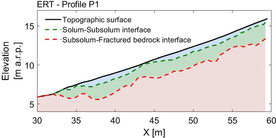
Electrical resistivity tomography (ERT) measurements were carried out for identifying the depth of the interfaces between solum-subsolum and subsolum-fractured bedrock. The ERT measurements were conducted along eight transects in the stream corridor and on the adjacent footslopes (Figure A1.1). We used a resistivity metre (IRIS Instruments, Syscal Pro 120, ten-channel) with multicore cables equipped with 120 stainless steel rod electrodes with 50 cm spacing increments. Data was processed following the approach outline by Gourdol et al. (2021) that surveyed the Weierbach catchment. The recorded resistivity data were pre-processed, removing values with a potential lower than 10 mV. The cleaned resistivity data was inverted using the Boundless Electrical Resistivity Tomography inversion code (Günther & Rücker, 2016). ERT images were processed to extract subsurface regolith layers through the derivative method. It was assumed that the subsurface regolith interfaces are located where the resistivity changes in space were at a maximum (Chambers et al., 2014). The changes in resistivity can be obtained by using the first or the second derivatives, targeting maximum gradients or zero values (Gourdol et al., 2021; Sponton & Cardelino, 2015). Zero values of the second derivative of the logarithm of resistivity were identified using Paraview (version 5.5.2, Kitware, Inc. Ahrens et al., 2005) to obtain the location of the interface between two different subsurface layers (Hsu et al., 2010). The two interfaces so obtained mirror the solum-subsolum-fractured bedrock morphology of the Weierbach regolith of previous studies (Glaser et al., 2016; Gourdol et al., 2021; Moragues-Quiroga et al., 2017). Starting from the location of the interfaces obtained from the ERT profiles, we derived the elevation of the solum-subsolum interface and the subsolum-fractured bedrock interface for every well and piezometer at the study site through linear interpolation (Figure A1.1 and Table A2.1). We were not able to clearly identify subsurface interfaces in the riparian wetland due to the relatively low resistivity of the Leptosols in this area. This is because the distinction between solum and subsolum is not reliable when resistivity contrast is low (Gourdol et al., 2021). To overcome this problem, a hand-drilling campaign was carried out to determine solum-subsolum-fractured bedrock interfaces in the riparian wetland (details in Data S1).
3.3 Analysis of precipitation events and groundwater flow direction
Precipitation was measured using a tipping bucket rain gauge located 3.5 km from the site. Individual events were defined with at least 1 mm of precipitation and separated by at least 2 h without precipitation. For every event, we calculated: groundwater response time (defined as the lag time between the beginning of the precipitation event and a vertical 1 cm rise of the water table), streamflow response time (defined as the lag time between the beginning of the precipitation event and an increase of 0.1 L/s of streamflow), total precipitation depth, event intensity, and number of days without precipitation prior to the event. For every continuously monitored well, we evaluated the correlation between level increase and the response time with the initial groundwater level and precipitation characteristics (i.e., depth, intensity and number of antecedent dry days). We correlated the spatial differences in the average groundwater response time and increase per well with the regolith depth above the fractured bedrock and with the distance from and elevation above the streambed using the Spearman rank correlation coefficient (Rs). Significance was evaluated with the Mann–Whitney test (significance level: p-value < 0.05).
We computed groundwater flow directions by assuming that they were equal to the slope of a planar groundwater table determined by three adjacent wells. We quantified the direction by angle α (degrees) on the xy plane (cf. Rodhe & Seibert, 2011). The stream is oriented with −72° on the xy plane (cf. Figure 2(b)). α-values pointing towards the stream channel indicate that the stream is gaining conditions, whereas α pointing away from the channel suggests losing conditions. The subsurface groundwater flow direction was calculated every 15 min. For the wells equipped with continuous water level loggers (Figure 2(a), 29 triangles), and for all wells every 2 weeks (Figure 2(b), 65 triangles). For every triangle we also derived the direction of the fractured bedrock fall line (defined as the direction on the xy plane [degrees] of the slope of fractured bedrock surface) and the direction of the surface topography fall line (defined as the direction on the xy plane [degrees] of the slope of the topographic surface) using the same approach used for obtaining the direction of the groundwater table. Data analysis has been conducted with Matlab R2020a (The Mathworks, Natick, MA).

4 RESULTS
4.1 Groundwater and streamflow dynamics
Streamflow varied widely (Figure 3, arithmetic mean of 6.5 L/s, median of 1.7 L/s, interquartile range of 9.1 L/s, St.Dev. of 11.52 L/s), with extended no-flow periods during summer (no discharge for a total of 194 days during the study period), persistent streamflow during winter and spring, and variable event responses. We defined three different hydrologic conditions (dry, intermediate, wet) based on streamflow and groundwater levels (shown as grey shades, Figure 3; details in Table 2) to classify groundwater behaviour.

| Period | Hydrologic classification | Fraction of time with streamflow (%) | Number of precipitation events | Total depth of precipitation (mm) | Precipitation depth per event (mm) | Precipitation inter-arrival time (days) | Duration of precipitation events (h) | |||
|---|---|---|---|---|---|---|---|---|---|---|
| Mean | St.dev. | Mean | St.dev | Mean | St.dev | |||||
| 25/07/2018–30/10/2018 | Dry | 4.97 | 18 | 111.8 | 6.21 | 9.43 | 4.54 | 5.41 | 5.01 | 6.92 |
| 30/10/2018–24/11/2018 | Intermediate | 26.05 | 12 | 57.3 | 4.77 | 6.25 | 1.99 | 2.52 | 5.39 | 3.52 |
| 24/11/2018–29/06/2019 | Wet | 100 | 94 | 584.6 | 6.22 | 9.07 | 2.26 | 4.51 | 7.1 | 8.28 |
| 29/06/2019–23/07/2019 | Intermediate | 36.18 | 0 | 0 | // | // | // | // | // | // |
| 23/07/2019–24/09/2019 | Dry | 4.71 | 19 | 102.5 | 5.39 | 5.02 | 3.00 | 5.21 | 4.79 | 4.78 |
| 24/09/2019–08/10/2019 | Intermediate | 46.87 | 17 | 113.2 | 6.66 | 7.23 | 0.45 | 0.49 | 6.66 | 6.57 |
| 08/10/2019–05/02/2020 | Wet | 100 | 71 | 523.7 | 7.37 | 7.78 | 1.29 | 1.88 | 9.29 | 7.71 |
We defined wet conditions when discharge Q exceeded 0 L/s for 14 consecutive days regardless the groundwater elevation in the wells.
Intermediate conditions were only defined when they immediately occurred before or after the wet conditions. Intermediate conditions were specified when Q = 0 or Q > 0 L/s lasted less of 14 consecutive days, and when the monitored groundwater in at least 17 (75%) of the wells was above the subsolum-fractured bedrock.
Dry conditions were specified when Q = 0 or Q > 0 L/s lasted less of 14 consecutive days and when the monitored groundwater in less than 17 (75%) of the wells was above the subsolum-fractured bedrock.
Dry conditions (dark grey shading, Figure 3, 28.7% of the observation period) (Table 2) had no-flow for 95.3% of the time. The average streamflow in this period was 0.01 L/s. Groundwater (Figure 3(b)) displayed flashy and short-lived increases after precipitation. The groundwater table in the east and west footslopes (wells 7W1 and 9W6, Figure 3(b)) showed larger increases and faster recessions than tables in the riparian wetland (well 9W6, Figure 3(b)). During intermediate conditions (light grey shading, Figure 3, 11.0% of the observation period, Table 2), precipitation occurred more frequently and with higher amounts; no-flow persisted for 67.4% of the time (Table 2) and average streamflow was 0.12 L/s. During wet conditions (white shading, Figure 3), which covered 60.3% of the observation period (Table 2), streamflow was persistent (average discharge was 10.8 L/s with a maximum of 118 L/s).
To quantify the drivers of groundwater dynamics, we analysed the average response time and increase after precipitation events for groundwater and streamflow (Figure 4). During dry conditions, a groundwater response was triggered in all wells by small precipitation depths (<3 mm for 21 of the 22 wells; median = 2.2 mm, min = 1 mm, max = 3.5 mm, Figure 4(a)). This groundwater rise occurred a few hours after the onset of precipitation (<3 h, for 17 of the 22 wells; median = 2.48 h, min = 1.21 h, max = 5.15 h, Figure 4(d)). If streamflow was generated following precipitation, it appeared several hours after the rise of the groundwater table (between 0.25 and 2.95 h; median = 1.75 h, Figure 4(g)). During dry conditions and before precipitation events (Figure 5(a)), the groundwater table in the footslopes was below the streambed elevation (Figure 5(d)) in the fractured bedrock (Figure 5(g)). The groundwater table in the riparian wetland was above the subsolum-bedrock interface and – for some wells – above streambed elevation (Figure 5(d),(g)). In response to precipitation events, groundwater in the footslopes rose rapidly from the fractured bedrock into the subsolum – and in a few instances – above streambed elevation. After events, the groundwater level decreased rapidly towards the pre-event level.


During intermediate conditions, the minimum precipitation depth necessary for a groundwater response was <3 mm for 21 of the 22 wells (median = 1.5 mm, min = 1.3 mm, max = 3.37 mm, Figure 4(b)). Groundwater rise usually occurred less than 5 h after the beginning of a precipitation event for most wells (median = 3.56 h, min = 2.17 h, max = 6.53 h; Figure 4(e)). In response to precipitation, streamflow increased (or re-appeared) almost synchronously with the groundwater table (Figure 4(h)). During intermediate conditions, the groundwater table was above the fractured bedrock and rose within the subsolum layer after the events and decreased to the pre-event level within 2–3 days (Figure 5(h)). The groundwater in the riparian wetland was always above the streambed elevation before and after precipitation events, while the groundwater in the footslopes was mostly at the level of the streambed (Figure 5(e)).
During wet conditions, the groundwater table was always above streambed elevation (Figure 5(f)) and in the upper subsolum (Figure 5(i)). The groundwater table variation in the footslopes mirrored streamflow variations (Figure 2(a),(b)), while the groundwater table in the riparian wetland was more stable with less frequent and smaller peaks (Figure 2(b)). The precipitation depth necessary to trigger an increase in the groundwater level was highest in wet conditions (median = 3.24 mm, min = 1.81 mm, max = 4.1 mm, Figure 4(c)) and the groundwater response to precipitation events was more delayed compared to dry and intermediate conditions (median = 5.58 h, min = 2.35 h, max = 12.68 h Figure 4(f)). In contrast to dry and intermediate conditions, streamflow response occurred before groundwater response (median = 4.54 h, min = 1.26 h, max = 11.41 h, Figure 4(i)). In the riparian wetland, the groundwater table reached the surface in several wells (8.5%, 6.8%, 14.6%, and 50.3% of the time for wells 7W2, 7W3, 9W3, and 10W2, respectively). Some wells displayed artesian behaviour for extended periods of time (46.5% and 14.9% of the time for wells 7W3 and 10W2, respectively).
We conducted a correlation analysis for every well to determine whether precipitation characteristics and initial groundwater table elevation drove temporal variability of groundwater dynamics in different hydrologic conditions (Figure 6 and Data S3). The increase in the groundwater level was always positively correlated with precipitation depth (Figure 6(a)), and it was positively correlated with precipitation intensity for the whole study period and for intermediate and wet conditions (Figure 6(b)). The increase in the groundwater level was also negatively correlated with the initial groundwater level for most wells during the whole study period (Figure 6(d)). We found no significant correlation between groundwater increase and number of antecedent dry days (Figure 6(c)). The observed groundwater response time was always negatively correlated with precipitation intensity (Figure 6(f)) and the correlation was significant for the whole study period and for intermediate and wet conditions. For the whole study period, the groundwater response time was also significantly positively correlated with initial groundwater levels for most wells (Figure 6(h)). We found no significant correlation between groundwater response time and precipitation depth or number of antecedent dry days (Figure 6(e,g)).

We conducted a correlation analysis to determine whether the regolith thickness and distance from and elevation above the stream channel drove spatial variability in groundwater dynamics for different hydrologic conditions. During wet conditions, the average groundwater increase and response time were significantly positively correlated with regolith thickness above the fractured bedrock and elevation above and distance from the streambed. During dry conditions, the average groundwater increase and response time were respectively significantly correlated with elevation above the streambed and regolith thickness above the fractured bedrock (Data S3).
4.2 Spatiotemporal dynamics of groundwater flow direction
α showed spatial patterns with clear differences between the east footslope, west footslope and the riparian wetland. The patterns are illustrated for two sets of 2 days using manual level measurements before and after precipitation events (Figure 7). The first example of 2 days relates to dry conditions (Figure 7(a),(c),(e)). Before the event (falling limb, 26 August 2019), α pointed towards the stream channel on the east footslope and towards the hillslope on the west footslope (Figure 7(e), red arrows). Observed groundwater levels were mostly below the streambed (medianGW_wells = 7.2 cm and medianGW_piezo = 11 cm below the streambed) with groundwater in the stream channel generally at the same level or below groundwater in the footslopes (e.g., the level differences between the piezometers 4P1 and the adjacent well 4W1 was ΔGW4P1-4W1 = −4.7 cm). In the riparian wetland, α pointed towards the stream channel. The event on 7 September led to an increase in the groundwater level throughout the study reach (medianGW_wells = 1.1 cm, medianGW_piezo = 1.8 cm below the streambed on 9 September 2019; Figure 7(a),(c),(e), blue arrows). As a result, groundwater in the streambed rose above the level of the adjacent groundwater in several sections (e.g., ΔGW4P1-4W1 = 15.3 cm) and α pointed towards the footslopes in some sections of the stream corridor (Figure 7(e)).

The second example relates to wet conditions (Figure 7(b),(d),(f)). Before the event (falling limb, 25 February 2019), the groundwater table was above the streambed elevation (medianGW_wells = 7.8 cm, medianGW_piezo = 3 cm above the streambed in the wells). Yet, groundwater in some piezometers was above that of the adjacent wells (e.g., ΔGW6P2-6W2 = 3.5 cm), and at the same level or below the streamwater level (e.g., ΔGW6P2-SW = −1 cm). α pointed towards the hillslope on the west footslope and in a few locations close to the stream channel on the east footslope (Figure 7(f), red arrows). However, α pointed towards the stream on the east footslope upstream of the stream riffle and in the riparian wetland. This occurrence of both gaining and losing conditions in different sections of the stream was not persistent during wet conditions. After a series of precipitation events (total precipitation = 49 mm between 1 and 8 March 2019) the groundwater level increased and α pointed towards the stream channel throughout the study reach (8 March 2019, medianGW_wells = 16.6 cm, medianGW_piezo = 5.2 cm above the streambed; Figure 7(f), blue arrows). Groundwater in the piezometers was generally below the adjacent groundwater in the footslopes (e.g., ΔGW6P2-6W2 = −6 cm) and at the same level or above the streamwater level (e.g., ΔGW6P2-SW = 0 cm). An exception was the east footslope close to the riffle, where local gradients pointed away from the stream channel.
The analysis of groundwater flow directions with continuously-monitored wells is generally consistent with the biweekly data and provided clear short-term dynamics of α and the duration of the gaining and losing conditions for different sections of the stream corridor (Figure 8). On the east footslope, α pointed towards the stream channel in dry, intermediate, and wet conditions in most triangles for most of the time (Figure 8(a),(d),(g)). However, during intermediate and dry conditions, α occasionally pointed away from the stream channel (Figure 8(a),(d)). On the west footslope, the groundwater flow direction towards the stream channel became relatively more important compared to the groundwater flow direction pointing away the stream channel with increasing wetness conditions (Figure 8(b),(e),(h); Tr2, Tr19). Here, spatial differences were observed in triangles closer to the stream, where α pointed mostly parallel (≃ − 72°) to the stream channel (Figure 8(b),(e),(h); Tr17), and in triangles closer to the riparian wetland, where α pointed constantly towards the stream channel (Figure 8(b),(e),(h); Tr4). In the riparian wetland, α nearly continuously pointed towards the stream channel for different hydrologic conditions (Figure 8(c),(f),(i)) with some exceptions close to the stream (cf. Triangle 22).

The continuously observed groundwater wells allowed us to capture the behaviour of α during the transition from dry to wet conditions (Figure 9(a)–(d)) and during events (Figure 9(e)–(l)). The transition was accompanied by a gradual change in α towards the stream on the east (Figure 9(b)) and west (Figure 9(c)) footslopes and partly in the riparian wetland (Figure 9(d)). α also varied between the directions of the fall line of the surface topography and the direction of the fall line of the factured bedrock surface for the majority of the continuously monitored wells.

The continuous measurements offered insights into event-based changes of α. During dry conditions, precipitation events were followed by sporadic re-appearance of the streamflow in the channel (from Q = 0 to Q > 0 L/s for 3 h Figure 9(a),(e)) and a shift of groundwater flow direction on the east footslope, with α pointing towards the stream between events and towards the hillslope after events (Figure 9(b),(g)). On the west footslope, α always pointed towards the hillslope (Figure 9(c)) and was almost perpendicular to the stream channel (α ~ −160°) after events (Figure 9(i)). During wet conditions, precipitation events were followed by an increase of streamflow (Figure 9(f)) and a more pronounced groundwater flow direction towards the stream. While this variation did not considerably change α on the east footslope (Figure 9(b),(h)), it caused a change in the groundwater flow direction on the west footslope. Here, α shifted from pointing towards the footslope during recessions to pointing towards the stream during and few days (up to 3 days) after events (Figure 9(c),(j)). In the riparian wetland, α always pointed towards the stream channel (Figure 9(d)) and approached the direction of the surface fall line after sporadic precipitation events in dry conditions (Figure 9(k)) and persistently during wet conditions (Figure 9(l)).
5 DISCUSSION
5.1 Drivers of near-stream groundwater dynamics
5.1.1 Role of depth-dependent storage capacity on groundwater response
We observed clear differences in groundwater response to precipitation between dry, intermediate, and wet conditions with the most pronounced and fastest increase of groundwater levels during dry conditions, and more delayed and less pronounced increases during wet conditions (Figure 4). Our results suggest that a decrease in porosity and storage capacity with depth act as critical controls on the average precipitation depth necessary to trigger a groundwater level increase and groundwater response times. This is supported by the Spearman correlation coefficients, which suggest that the deeper the initial groundwater table is, the faster and the higher the groundwater table response to precipitation (Figure 6(d),(h), Data S3). This is due to the subsurface layering in the Weierbach, with high porosity and storage capacity in the solum and subsolum, and lower porosities and storage capacity in the fractured bedrock below (Glaser et al., 2016; Martínez-Carreras et al., 2016). When groundwater levels were located in the low porous fractured bedrock (~10%–15%, Table 1), the same amount of precipitation led to a more pronounced increase compared to higher groundwater stages where porosity was higher (15%–30% in the subsolum and 45%–61% in the solum, Table 1).
The role of variable storage capacities in the subsurface has been highlighted at other catchments, where groundwater response was faster and more pronounced in locations characterised by soils with low storage capacities compared to deeper soils with higher storage capacities (Penna et al., 2015; Rinderer et al., 2016; Rinderer et al., 2017; Rodhe & Seibert, 2011). These studies showed a spatial effect of storage capacity leading to a spatially non-unison response across hillslopes. Adding to this, we showed that the vertical decrease in storage capacity leads to clearly different groundwater responses between events in different hydrologic conditions. Our results highlight the relevance of covering the full range of hydrologic conditions in order to capture the effect of a decrease of subsurface storage capacity with depth on seasonally different groundwater responses.
5.1.2 Role of precipitation characteristics on groundwater response
The increase of the groundwater level following events was significantly correlated to precipitation depth for dry, intermediate, and wet conditions and for the entire study period (Figure 6(a), Table A3.1). Combined with previous findings, our results underline the dominant role of precipitation depth on groundwater level increase in humid mountain hillslopes, regardless of the topographical location and the geological settings (Dhakal & Sullivan, 2014; Fannin et al., 2000; Penna et al., 2015; Rinderer et al., 2016). Precipitation intensity controlled the response time and increase of groundwater levels after events for the full observation period, and for wet and intermediate conditions, however, it was not correlated to groundwater increase and response time for most of the wells in dry conditions (Figure 6(b),(f)). This may be because low storage capacities in the fractured bedrock caused a quick rise in the groundwater, regardless of the precipitation depth and intensity. Yet, groundwater levels were not sustained above the fractured bedrock layer beyond a week, which is likely due to lacking contributions from upslope to the stream corridor during dry conditions, since they are threshold-driven (Martínez-Carreras et al., 2016). However, during intermediate and wet conditions, the precipitation depth necessary for a groundwater increase is higher due to the higher porosity of the subsurface near the surface. At this stage, precipitation intensity controls the time needed until storage is filled. This result contradicts previous findings (Dhakal & Sullivan, 2014; Fannin et al., 2000; Penna et al., 2015), which reported groundwater response to be uncorrelated with rainfall intensity. This might be explained by the different hydrologic conditions at our study site causing the groundwater table to lie in layers of the regolith with storage capacities decreasing with depth, which might not occur in hillslopes with a thicker and less stratified regolith (Penna et al., 2015). However, our observations are in agreement with the observations of Rinderer et al. (2016), who reported a lower importance of precipitation intensity for groundwater response time at sites characterised by a low storage deficit compared to sites with a higher storage capacity. Our observations highlight the importance of monitoring events across wetness states to decipher the transient role of precipitation depth and intensity on groundwater response times.
5.1.3 Role of regolith thickness above the fractured bedrock on groundwater response
The observed spatial differences between groundwater level increase and response times for different wetness states allowed us to highlight the temporally changing relevance of regolith thickness on groundwater dynamics. Groundwater response time following precipitation was correlated to the storage capacity above the fractured bedrock (Table A3.3) when groundwater level is above the bedrock surface (i.e., wet conditions). The influence of distance from and elevation above the stream on the response times of the groundwater level (Table A3.3) is explained by increasing regolith thickness with the distance from the stream (Table A2.1). Our results for wet conditions are consistent with other studies reporting a correlation between asynchronous groundwater response and distance from the stream, and regolith thickness above the fractured bedrock (Haught & Van Meerveld, 2011; Montgomery et al., 1997; Penna et al., 2015; Rinderer et al., 2017; Seibert et al., 2003). The evaluated correlations also indicate that groundwater located in the shallow regolith near the stream had a less pronounced groundwater response after events than groundwater located in wells further from the stream. This can be explained by the storage capacity in the regolith of the Weierbach catchment, which was found to strongly decreases with depth (Gourdol et al., 2021; Martínez-Carreras et al., 2016; Wrede et al., 2015). Therefore, a certain increase in the groundwater in the upper part of the regolith would require more water compared to the same increase in the lower regolith. As a result, groundwater in shallower soils close to the stream quickly rose into the upper and more porous soil and displayed a lower increase than groundwater further from the stream. This result is consistent with observations at other sites, where the water table rose more in locations characterised by thicker soils further from than stream than in locations characterised by shallower soils (Penna et al., 2015).
When the groundwater level is below the fractured bedrock surface (i.e., dry conditions), the derived correlations indicate that groundwater further from the stream responds with a delayed and less pronounced increase compared to groundwater closer to the stream (Table A3.3). This result can be explained by inflow from the stream channel into footslopes. This is also consistent with groundwater levels below the dry streambed, which increased above the adjacent groundwater after precipitation events (Figure 7(e)).
During intermediate conditions, the correlation analysis was not able to decipher different drivers controlling the groundwater dynamic in the system (Table A3.3). This might be explained by the fact that the increase of the groundwater table above the fractured bedrock is neither in unison in time nor uniform in space during the transition from dry to wet conditions (and vice versa). Therefore, the groundwater dynamic for some wells might be controlled by regolith depth, as observed during wet conditions, while the groundwater table response to events might be controlled by streamwater inflow for other wells, like during dry conditions.
5.2 Drivers of near-stream groundwater flow directions depending on hydrologic conditions
5.2.1 Role of upslope-footslope connectivity and streamwater level
The more pronounced groundwater flow direction observed towards the stream channel with increasing wetness conditions can be explained by seasonal groundwater dynamics in the hillslopes. In the Weierbach catchment, high evapotranspiration in summer depletes storage in the regolith (Glaser et al., 2016) and groundwater tables in the hillslopes decrease into the fractured bedrock (Rodriguez & Klaus, 2019). During the wet-up, the groundwater table rises across the hillslope into more conductive layers and contributes increasingly to streamflow (Rodriguez & Klaus, 2019). Despite the lack of an extended groundwater monitoring network across hillslopes, the groundwater flow direction observed towards the stream channel, together with previous modelling results (Glaser et al., 2020), indicate persistent hydrologic connectivity between near-stream and upslope groundwater during wet conditions. This interpretation is in agreement with several studies on hydrological connectivity in different landscapes, which consistently found near-stream groundwater flow direction pointing towards the stream when the inflow from upslope locations maintained high levels of near-stream groundwater (Rodhe & Seibert, 2011; van Meerveld et al., 2015; Vidon & Hill, 2004).
However, α did not point uniformly towards the stream channel during wet conditions, and in some sections of the reach, groundwater flow direction pointed towards the stream channel only after precipitation events (Figures 7(f) and 8(b),(c)). Here, groundwater flow direction shifted from pointing towards the stream after events to pointing towards the footslopes during recessions in wet and intermediate conditions. This result suggests, together with the decrease of near-stream groundwater below streamwater level, a reduced or lack of groundwater inflow from the hillslopes towards the stream corridor and local streamwater inflow towards the footslopes. The spatial differences of groundwater flow direction observed in the near-stream domain suggest an asynchronous connection and disconnection between upslope groundwater and footslope groundwater along the stream corridor. This result might be explained by properties of the hillslopes, such as moisture conditions (Penna et al., 2011) and water table elevation along the hillslope (Jencso et al., 2009; Ocampo et al., 2006).
Differences of transpiration driven by aspect were shown to be minor in the Weierbach catchment (Schoppach et al., 2021). Therefore, aspect is unlikely to explain the observed different groundwater dynamic between the east and west footslope. In addition to aspect, the role of upslope contributing area was tested (not shown here) for explaining different groundwater dynamic due to hillslope water balance. The results showed higher upslope contributing area for the west footslope compared to the east footslope (data not shown), which would suggest higher water flows and more pronounced groundwater gradients towards the stream channel on the west footslope. However, the observations are contrary to this with more persistent groundwater gradients towards the stream at the east footslope compared to the west footslope. Thus, the observed different flow groundwater gradients in the east and west footslopes during wet conditions and the asynchronous connection and disconnection between upslope groundwater and the footslopes are likely driven by bedrock topography in the hillslopes (Blume & van Meerveld, 2015; Hutchinson & Moore, 2000; van Meerveld et al., 2015) or by localised preferential flowpaths in the subsolum and in the fractured bedrock (Gabrielli et al., 2012; Glaser, Jackisch, Hopp, & Klaus, 2019; McGuire & McDonnell, 2010). However, since we currently have no additional information on these factors, we cannot address their influence on the observed spatiotemporal development of water flowpaths during wet conditions.
Groundwater flow direction pointing towards the footslopes has also been observed at alluvial sites due to an increase in streamwater level after events (Dudley-Southern & Binley, 2015; Heeren et al., 2014; Vidon, 2012; Vidon & Hill, 2004). Adding to the existing body of literature, our work highlights the occurrence of short- and long-lasting periods where groundwater flow direction also pointed away from the stream in steep-sloping (>5%) footslopes, while this was previously shown mostly in gentle-sloping (<5%) alluvial planes (Vidon & Hill, 2004). However, our results are not in agreement with other studies where the lack of groundwater inflow from the upslope was followed by near-stream groundwater flow direction pointing parallel to the stream channel with no potential for streamwater-groundwater mixing (Rodhe & Seibert, 2011; Vidon & Smith, 2007). These different results can be driven both by diverse properties ruling upslope-footslope connectivity in different catchments (Jencso & McGlynn, 2011) and also by the limited number of observations that previous studies relied on. Indeed, if we had based our interpretations only on a few wells in the east footslope, we would have also concluded that a lack of groundwater inflow from the upslope was followed by near-stream groundwater gradients pointing parallel to the stream during the dry-out. Therefore, our work highlights the importance of a spatially dense monitoring network in capturing the marked variability characterising streamwater-groundwater mixing.
5.2.2 The role of surface topography and anisotropic hydraulic conductivity of the fractured bedrock
During dry conditions, groundwater on the west and east footslopes decreased below the streambed into the fractured bedrock, and streamflow ceased (Figure 5(d)). At this stage, the groundwater flow direction showed a diverse pattern and pointed away from the stream at some locations and towards the stream at others (Figure 7(e)). This might be explained by a strong anisotropic hydraulic conductivity of the fractured bedrock. The weathering of bedrock can be heterogeneous, leading to the presence of preferential flowpaths (Gabrielli et al., 2012) and local changes in hydraulic conductivity (Hopp & McDonnell, 2009), resulting in spatial differences in the groundwater table (Welch & Allen, 2014). Moreover, bedrock fractures do not necessarily imply connectivity between wells and we do not necessarily expect the groundwater flow to exactly follow the observed gradients. This is reflected in Darcy's law if the conductivity tensor has large off-diagonal coefficients. The impact of fractured bedrock on groundwater flow directions is also evident once the groundwater rises above the fractured bedrock, then the groundwater table direction approaches the fractured bedrock fall line. This is apparent after precipitation events in dry conditions, when groundwater in some stream sections rose above the adjacent groundwater (Figure 7(e)), groundwater flow direction pointed towards the bedrock depression in the footslopes, and α approached the fractured bedrock fall line after events at several locations (Figure 9(b),(c),(g),(i)). These results are in line with observations in hillslope studies that showed that groundwater flow direction reflected the bedrock fall line during dry conditions (Hutchinson & Moore, 2000; van Meerveld et al., 2015). However, the information available on α in intermediate and wet conditions also demonstrated no significant correlation between α and the groundwater elevation above the fractured bedrock (results not shown). This is probably because inflow from upslope groundwater and the stream channel to river corridor groundwater quickly fills the bedrock depressions in wetter conditions, interrupting their influence on the groundwater flowpaths.
5.3 Implications for runoff generation and hydrological connectivity
Without additional data on groundwater flow direction, one may have interpreted the observed response of groundwater before streamflow response in dry conditions at the study site as groundwater contributing to streamflow generation. Such an interpretation would be in agreement with hillslope-stream connectivity studies, which concluded that streamflow generation is driven by groundwater inflow when groundwater responds to events before streamwater (Beiter et al., 2020; Haught & Van Meerveld, 2011; Rinderer et al., 2016). However, α and the detailed pattern of the groundwater level, that was consistently below the streamwater level, clearly showed that groundwater flow direction pointed towards the hillslope during and after precipitation events in dry conditions. This is evidence for the lack of groundwater contributions to streamflow generation in the study reach.
α and groundwater level above the streamwater level jointly revealed that groundwater contributes to streamflow generation both before and after precipitation events during wet conditions in most of the study reach. This is despite the fact that a response of groundwater after streamwater was previously linked to a lack of groundwater contribution to the streamflow generation (Beiter et al., 2020). The nearly instantaneous streamflow response in the Weierbach following precipitation largely consists of event water in dry and wet conditions (Wrede et al., 2015). This has commonly been interpreted as surface runoff generated in saturated areas or by direct precipitation in the stream channel (Glaser et al., 2016; Rodriguez & Klaus, 2019; Schwab et al., 2018) and is consistent with the spatial extent of saturated areas (Glaser et al., 2020) and the observations in the current study.
The high spatial density and high-frequency observations across hydrologic conditions in this study showed the potential pitfalls of using only one or a few wells for characterising runoff generation or hydrological connectivity. Using groundwater flow direction proved useful to avoid misinterpretations of hillslope-stream connectivity derived from time lags, as the lag time between the streamwater and groundwater response to events was interpreted contrary to our results in the same hydrogeological setting of the Luxembourg Ardennes (e.g., Beiter et al., 2020).
6 CONCLUSIONS
The dynamics of groundwater level and of groundwater flow direction were analysed in a headwater stream reach to evaluate temporal drivers for the streamwater-groundwater exchange. The groundwater response to precipitation events was clearly different in dry and wet hydrologic conditions. Correlation analysis based on groundwater response time, groundwater level increase, and precipitation characteristics (depth and intensity) showed that differing groundwater response to events for dry, intermediate, and wet conditions are controlled by the decreasing storage capacity with regolith depth. Precipitation depth, precipitation intensity, and regolith depth above the fractured bedrock also played a significant role in the groundwater response time and increase after events in wet conditions, while, during dry conditions, only the precipitation depth and water inflow from the streambed towards the footslopes controlled the groundwater increase after events.
Of particular interest is our finding that the groundwater gradients might point towards the footslopes in some sections of the reach and, at the same time, groundwater flow direction can point towards the stream channel in other sections of the reach, due to the interplay of different drivers both in wet and dry hydrologic conditions. The results presented in this study suggest that during dry hydrologic conditions the groundwater flow direction is controlled by the strong anisotropy in the hydraulic conductivity of the fractured bedrock and, once the water table lies above the fractured bedrock layer, by the direction of the fractured bedrock fall line. With increasing wetness conditions, the influence of bedrock topography was not apparent and near-stream groundwater flow directions were controlled by the competing influence of upslope-footslope connectivity and the streamwater level. Our results suggest that triggering of upslope-footslope connectivity in wet hydrologic conditions controlled the groundwater flowpath towards the stream channel. However, in the same hydrologic conditions the reduced or ceased groundwater inflow from upslope location towards the stream also let near-stream groundwater to lie below the streamwater level, causing the local inflow of streamwater into the near-stream groundwater and flow reversals towards the hillslopes.
While the lag time between groundwater and streamflow response to events can be used as indicator for groundwater contribution to streamflow generation and hillslope-stream connectivity, the observed groundwater flow directions were important to avoid result misinterpretation and allowed us to decipher different streamflow-generation processes in dry and wet conditions. The water flowpaths observed have important implications for solutes, nutrients and dissolved oxygen transport in the stream corridor with a strong potential for the development of hot-spots and hot-moments both in dry and wet hydrologic conditions. In conclusion, the results presented in this work offer new insights into the spatial heterogeneity and the time-variant role that different drivers exert on stream-groundwater exchange across a wide variety of precipitation events and hydrologic conditions. Additionally, our results highlight the pivotal importance of long-term observations in the stream corridor domain, since the lack of spatially-dense and high-frequency measurements can cause misinterpretation in the streamflow generation process, streamwater-groundwater exchange and hillslope-stream connectivity.
ACKNOWLEDGEMENTS
This work was supported by the funding from the Luxembourg National Research Fund (FNR) for doctoral training (PRIDE15/10623093/HYDRO-CSI). We would like to acknowledge the financial support of the Austrian Science Fund (FWF) as part of the Vienna Doctoral Programme on Water Resource Systems (DK W1219-N28). We thank Laurent Gourdol for providing the ERT surveys and analysing the resistivity data. We also thank Jean-François Iffly, Jérôme Juilleret, and Laurent Gourdol for their help in the installation of the monitoring well network and Cyrille Tailliez for the theodolite surveys. We thank Marta Antonelli, Samuele Ceolin, Ginevra Fabiani, Barbara Glaser, Christopher Hissler, Adnan Moussa, Laurent Pfister, and Nicolas Rodriguez for their fruitful input and discussions.
Open Research
DATA AVAILABILITY STATEMENT
The data that support the findings of this study are available from the corresponding author upon request.