Volume 3, Issue 2 pp. 88-100

ORIGINAL ARTICLE

Open Access

The novel hierarchical clustering approach using self-organizing map with optimum dimension selection

Kshitij Tripathi,

Corresponding Author

Kshitij Tripathi

[email protected]

orcid.org/0000-0003-3226-8717

Department of Computer Applications, The Maharaja SayajiRao University of Baroda, Vadodara, Gujarat, India

Correspondence Kshitij Tripathi, Department of Computer Applications, The Maharaja SayajiRao University of Baroda, Vadodara, Gujarat 390002, India.

Email: [email protected]

Contribution: Methodology (equal), Software (equal), Writing - original draft (equal), Writing - review & editing (equal)

Search for more papers by this author

Kshitij Tripathi,

Corresponding Author

Kshitij Tripathi

[email protected]

orcid.org/0000-0003-3226-8717

Department of Computer Applications, The Maharaja SayajiRao University of Baroda, Vadodara, Gujarat, India

Correspondence Kshitij Tripathi, Department of Computer Applications, The Maharaja SayajiRao University of Baroda, Vadodara, Gujarat 390002, India.

Email: [email protected]

Contribution: Methodology (equal), Software (equal), Writing - original draft (equal), Writing - review & editing (equal)

Search for more papers by this author

First published: 11 April 2024

https://doi.org/10.1002/hcs2.90

Share a link

Email
Wechat
Bluesky

Abstract

Introduction

Data clustering is an important field of machine learning that has applicability in wide areas, like, business analysis, manufacturing, energy, healthcare, traveling, and logistics. A variety of clustering applications have already been developed. Data clustering approaches based on self-organizing map (SOM) generally use the map dimensions (of the grid) ranging from 2 × 2 to 8 × 8 (4–64 neurons [microclusters]) without any explicit reason for using the particular dimension, and therefore optimized results are not obtained. These algorithms use some secondary approaches to map these microclusters into the lower dimension (actual number of clusters), like, 2, 3, or 4, as the case may be, based on the optimum number of clusters in the specific data set. The secondary approach, observed in most of the works, is not SOM and is an algorithm, like, cut tree or the other.

Methods

In this work, the proposed approach will give an idea of how to select the most optimal higher dimension of SOM for the given data set, and this dimension is again clustered into the lower actual dimension. Primary and secondary, both utilize the SOM to cluster the data and discover that the weight matrix of the SOM is very meaningful. The optimized two-dimensional configuration of SOM is not the same for every data set, and this work also tries to discover this configuration.

Results

The adjusted randomized index obtained on the Iris, Wine, Wisconsin diagnostic breast cancer, New Thyroid, Seeds, A1, Imbalance, Dermatology, Ecoli, and Ionosphere is, respectively, 0.7173, 0.9134, 0.7543, 0.8041, 0.7781, 0.8907, 0.8755, 0.7543, 0.5013, and 0.1728, which outperforms all other results available on the web and when no reduction of attributes is done in this work.

Conclusions

It is found that SOM is superior to or on par with other clustering approaches, like, k-means or the other, and could be used successfully to cluster all types of data sets. Ten benchmark data sets from diverse domains like medical, biological, and chemical are tested in this work, including the synthetic data sets.

Abbreviations

ANNs: artificial neural networks
ARI: adjusted randomized index
CH: Calinski–Harabasz
DBSCAN: density-based spatial clustering of applications with noise
FCM: fuzzy C-means
HSOM: hierarchical self-organizing map
SOM: self-organizing map
ST: Silhouette
WDBC: Wisconsin diagnostic breast cancer
WM: weight matrix

1 INTRODUCTION

Data clustering is one of the main fields of data mining that falls under unsupervised learning. Clustering techniques try to discover the group of similar instances, and their result is the optimum number of these groups, provided all these groups do not have any common instances. There are various techniques available for data clustering that include k-means, fuzzy C-means (FCM), and Kohonen self-organizing maps (SOMs). It is seen that artificial neural networks (ANNs) are opaque (they do not reveal any rules) but have a strong potential to understand the intricacies of data. They have the unreasonable capability to establish a relationship between the input and output data using mathematical techniques where the data format must be numeric. ANNs deliver excellent results in the classification of data [1-3], which come under supervised learning. In this article, we explore Kohonen's SOM as well as their one- (1D) and two-dimensional (2D) clustering spaces and observe that they are also capable of giving excellent results in clustering. For this, we consider the Silhouette (ST) or Calinski–Harabasz score (CH), as the case may be, to select the optimum configuration of SOM. The ST and CH scores help in evaluating whether the given number of clusters is accepted to be optimal or vice versa. The experiments are performed on the preprocessed data (min–max normalized), which increases the chances of getting improved results. There is no removal of attributes or instances in any experiment, and still high accuracies are obtained on the data sets involved. The objective of this work is to unleash the power of ANNs, or more specifically, SOMs, and demystifies promising results. Also, it is illustrated that the weight matrix (WM) of SOM is very meaningful in giving better results.

1.1 ST score

It is a measure of how each object in its cluster is closest in comparison to other neighboring clusters. Its value lies between −1 and +1. It is defined as

\text{ST}[O]=\frac{[b(o)-a(o)]}{\max [b(o),a(o)]},

()

where b(o) is the mean distance of the object (o), with respect to its closest neighboring cluster, and a(o) is the mean distance of the object (o), with respect to all the other objects in the cluster A high ST score value signifies that the object is well-matched to its own cluster and poorly matched to neighboring clusters.

1.2 CH score

It is also called the variance-ratio criterion. It is defined as

\text{CH}\,=\frac{{V}_{\text{bc}}}{{V}_{\text{wc}}}\times \frac{N-k}{k-1},

()

where V_bc is the overall between-cluster variance, V_wc is the overall within-cluster variance, k is the number of clusters, and N is the number of observations. The optimal number of clusters is the solution with the highest CH index value.

1.3 Literature review and related work

Clustering of data is an unsupervised learning technique that tries to assign the appropriate class labels to unclassified data instances. The applications of clustering include document classification, image classification, medical data analysis, and biological classification. There are various methods for clustering available in the literature [4, 5], and they are discriminated against based on either the intrinsic structure of the data to which they are applied or on the methodology itself. In the former case, the phenomenon observed is that the clusters are of an arbitrary shape, which may be spherical or oval, while some are “S” shaped. In the latter case, the approach of the clustering technique is different; some are partitioning based or hierarchical, while others are density or grid based. The partitioning algorithms are distance-based (generally Euclidean) and use the mean or the medoid to represent the cluster center, like, the k-means algorithm [5]. Hierarchical-based algorithms decompose the data into multiple levels, like, BIRCH and Chameleon. The density-based algorithms work by connecting the regions with a high density, like, density-based spatial clustering of applications with noise. Grid-based algorithms partition the data by constructing a multiresolution grid. Some other popular algorithms are SOM, FCM, and probability clustering [5]. The FCM is based on the centroid of the clusters, whereas the probability clustering is based on the density function. The SOM is based on ANN, and the most distinguishing property of the SOM is its ability to cluster the data into 2D space, which is not possible in the case of one of the most widely used k-means algorithms. Another advantage of SOM is that they can cluster the data into arbitrary shapes. This work considers the two most common clustering evaluation techniques, that is, the ST [6] and CH [7] scores, to obtain the optimum value for a number of clusters. The SOM algorithm is explored in this article with the help of the ST [6] and the CH score [7]. The above scores come under the intrinsic methods and are used when the ground truth of the data set is not available. SOM is proposed by Kohonen to map the data patterns into a multidimensional grid of neurons [8-10]. Two-dimensional grid structures are most notable, and dimensions greater than two are not frequent in the existing clustering literature. Various researchers applied the SOM to the data clustering tasks that belong to the different domains. Lampinen et al. apply a hierarchical self-organizing map (HSOM), which is a multilayer version of SOM and is used as an image analysis system [11]. Wu and Chow use the local clustering validity index based on the intercluster and intracluster density, which is a two-level algorithm [12]. In the second level, it applies the agglomerative hierarchical clustering method to data sets, like, Iris, the 15D synthetic data set, and gene expression data. Drigas and Vrettaros used the clustering technique as an e-content retrieval tool [13]. Drigas et al. apply SOM to the document data sets for clustering the documents based on their semantic similarities and call it WEBSOM. Argyrou uses the SOM algorithm as a graph–theoretical approach to cluster hierarchically and apply it to the zoo data set [14]. Nidheesh et al. utilize the improved deterministic k-means clustering approach to forecast the cancer subtype based on gene expression information [15]. They used the gene expression data set GEO, which is a group of five data sets in addition to five other data sets, that is, Iris, Wine, Seeds, New Thyroid, and Wisconsin Diagnostic Breast Cancer (WDBC). Their work also displays results based on the adjusted randomized index (ARI) using SOM on the above data sets. Ambroise and Govaert have done work on constrained clustering using probability theory [16]. Jain has described k-means to solve the data clustering tasks [17]. Fränti and Sieranoja apply k-means to some benchmark clustering data sets, including synthetic data [18]. Ray et al. [19], Nguyen et al. [20], Ripan et al. [21], Tarekegn et al. [22], and Chen et al. [23] have used various clustering techniques for different applications, and some of them also apply SOM. Townsley et al. [24] and Wang and Zhang [25] apply machine learning algorithms to medical data sets for classification purposes.

1.4 Research contributions

The proposed approach guides the selection of the best 2D configuration of the SOM, which then maps into an actual number of clusters and proves the candidature of the SOM in the field of data clustering is invincible. Medical or healthcare data frequently requires clustering to segregate records to group similar types of patients or populations, so the proposed approach helps do the same and can group high-dimensional data (a greater number of features or attributes) into an optimum number of clusters or assign labels to instances with high accuracy. The WM is also found to be meaningful, as reflected in the proposed approach. The proposed approach reflects that the SOM performs more efficiently than in the past and proves that an ANN could be used for clustering the data as a single technique (a hierarchical approach would be better) using the SOM.

1.5 Architecture of SOM

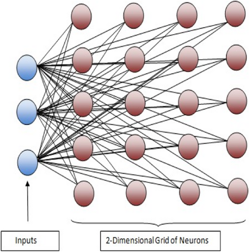
SOM, as shown in Figure 1, is usually a 2D grid of neurons, where each neuron itself is a microcluster, though high-dimensional SOM is also possible. All the edges through which neurons are connected to the input layer have weights associated with them. These weights are updated after each epoch, where an epoch means one cycle of training, and all the instances are applied as input once. SOM learns to classify the data instances based on competitive learning. In competitive learning, during the training phase, either one or a few neurons are activated by applying the input vector. The neuron that has the largest activation is called the winning neuron, and the corresponding instance is assigned to it. Also, competitive learning is localized learning in which the updating of weights is done only for active neurons. The various topologies available are grid-top, hex-top, or rand-top, and the arrangement of neurons is either grid, hexagonal, or random. The steps of the SOM are given in Algorithm 1. All experiments in the current work are carried out using Matlab, and all the data filtering tasks are done in Excel. In Matlab, all default values are accepted, like, the training algorithm, neighborhood function, and random seed, except the configuration (dimension) of SOM, which is finally selected based on the ST or CH score. The epoch limit lies from 500 to 1350.

Details are in the caption following the image — **Figure 1**
Open in figure viewer PowerPoint

Architecture of self-organizing map.

2 METHODS

The proposed approach could be summarized into five steps (Algorithm 2). Figure 2 describes the pictorial view of the proposed approach. In the proposed algorithm (HSOM), the data set is first converted into min–max normalized form. The prepared data set is then mapped by SOM into dimensions ranging from 2 × 2 (4 neurons) to 10 × 10 (100 neurons), where each neuron corresponds to a single cluster, that is, each neuron incorporates one or multiple numbers of instances. All the corresponding weight matrices are saved as buffers for further processing. This WM now acts as the input data set, and SOM is again checked to see which 2D map (WM) is best. The best WM selected is again clustered into an actual number of dimensions using SOM itself, as it is a type of mapping of WM into an optimum number of clusters and their corresponding records (instances) too. It is to be noted that each neuron is associated with some specific number of records (data instances). It might be possible that the optimized higher dimension is not 2D but may be 1D (like 1 × 5, 1 × 10, or vice versa), but will be clustered into a lower dimension that is 1 × 2, or 1 × 3, or 1 × 4.

Before doing all the tasks, it is mandatory to find the optimum value (actual value) of the number of clusters for the particular data set. The SOM is executed first on the raw data, and both the ST score and the CH score are calculated to determine the peak corresponding to different values of O_c (generally ranging from 2 to 8 for most of the data sets). This O_c, corresponding to peak scores (CH or ST), will be the value for the optimum number of clusters in the data set. The elbow method could also be used to find the optimum (actual) value of a number of clusters in the data set. Figure 3 displays and explains the graph patterns after plotting them, assuming a number of clusters on the x-axis and a CH or ST score on the y-axis. It is to be noted that the ideal value of the ST score is 1. If the ST score on WM corresponding to the value of O_c is 1, and this O_c is determined from the raw data according to procedures 1 and 2, then this WM and its dimension are considered optimum.

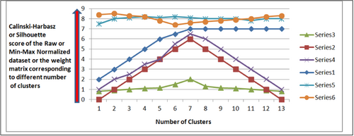
It is observed that the clustering evaluation techniques for finding the optimum number of clusters, like, ST and CH scores, do not give the same results on the given data set, and their score sensitivity is different for the different data sets. If we draw a 2D graph between the number of clusters (generally ranging from 2 to any arbitrary value) as the x-axis and their ST or CH score as the y-axis, then the graph patterns may be ascending, descending, or horizontal for the ST but give a local maximum for CH or vice versa (Figure 3). Therefore, in this work, both scores for a given data set are computed, and we consider the score that gives the global maxima with the sharpest peak (Figure 4). After getting the value for the optimum number of clusters (O_c) on the raw data, we consider the same score strategy and evaluation technique for later phases (when the WM acts as input). Finding the most promising higher-dimensional (HD) SOM configuration is also a challenging task. Procedures (1 and 2) are used to select the most optimum HD configuration using the corresponding WM. After executing Procedures 1 and 2, an optimum HD weight configuration (matrix) is selected. The WM obtained is explored in the proposed approach as it fairly describes the intricacies of the data set. The dimension of this WM depends on the number of neurons and the number of attributes in the data set. For example, if the configuration of the SOM is i × j, then it is obvious that there are i × j neurons (microclusters) in the given configuration, and therefore i × j rows and at columns are in the WM, where a_t is the number of attributes in the data set. It is observed that very few all the HD SOM configurations (WM) give a local maximum at the same optimum value, which is also the optimum number of clusters. So first, we inspect enough HD configurations and select the best configuration by looping such that their global maxima lie on the value (O_c) that also reflects an optimum number of clusters and has the sharpest peak. If the number of attributes without class attribute in the data set is a_t and the number of neurons in the SOM is n_e, then each of these attributes separately contributes its weights to all neurons. On the other side, all instances of the data set are clustered around these neurons (microclusters); hence, each neuron encompasses one or more instances of the data set. After finding the best HD configuration and the respective WM, SOM is again executed (and that is the reason to call it HSOM), treating this WM as a data set and mapping the microclusters into final clusters. The data indices assigned to the HD WM are finally mapped to lower dimensions (O_c).

Algorithm 1. SOM.

1: Let {x₁, x₂, x₃, …, x_n} are training vectors each of size #a_t rows and column

2: Let grid of neurons is of configuration i rows and j columns that is i × j neurons

Are there in the map

3: Let W_mn be the weight matrix associated with inputs to an every neuron (it is initialized by random number seed)

4: Let α be the initial learning rate

5: Let f (e, r) be the neighborhood function that determines the rate of change of neighborhood around the winner neuron after each iteration e, and r is the radius of neighborhood function

6: Let d be the Euclidean distance between the input vector x and the neuron with given weight vector w_ct where d (x, w) = ||x_t–w_ct||

7: Repeat

8: Determine d for all w belong to W_mn SOM will search for the winner neuron using the minimum d that is also called best matching unit (BMU) and weights are also adjusted (updated) after obtaining the winning neuron by applying the neighborhood function using the equation w_ct = w_ct + α (e) f (x (e)˘w_ct (e)) (for all w_ct) (where e is the current iteration)

9: Decrease α and r

10: Until {the specified number of epochs or other specified threshold value is reached}

Algorithm 2. Hierarchical SOM (HSOM).

Step 1: Convert the original data set into its min–max normalized form (D_n).

Step 2: Determine the best suitable value for O_c (where O_c = Optimum number of clusters) from the raw data using ST or CH score based on procedure 1 and 2. The other approaches like Elbow method can also be used for finding the value of optimum number of clusters.

Step 3: Treating D_n as input data set, Run SOM with dimensions ranging from 1. .10 × 2. .10 and save all its corresponding weight matrices in buffer.

Step 4: Treating these weight matrices one by one as input data set, run SOM on each of them,and discover the weight matrix that gives sharpest ST or CH score at O_c.

Step 5: Again run the SOM with dimensions of (1 × O_c) treating the discovered weight matrix obtained in step 4 as input dataset.

After step 5 the data set is finally clustered.

Procedure 1. Determinethe ST and CH Score for the given dataset corresponding to the different values of optimum number of clusters (2 to maxO_c) (D (Without the Class attribute), x (2 ≥ x ≤ maxO_c))

D_t = D

Let x

\in

Z such that 2 ≥ x ≤ maxO_c and maxO_c be any arbitrary value

For x = 2 to maxO_c

Eval1 [D_n,x] = STscore (D,x)

Eval2[D_n,x] = CHscore (D,x)

End

Output: Arrays of the ST (Eval1) and CH score (Eval2) on D

Where x lies between 2 to maxO_c

End procedure

Procedure 2. Determine the best score among ST and CH score for the given dataset from the graph obtained in procedure1 and find the value of optimum number of clusters (O_c)(Eval[], Eval2[])

Goal: The graph must be sharpest at x equal to O_c and is global maxima

Input: Eval1 and Eval2 (Arrays of ST score and CH score) of D for values of x(2 ≥ x ≤ maxO_c)

Output: One of the ST or CH score with corresponding x equal to O_c

Let x

\in

Z such that 2 ≥ x ≤ maxO_c and maxO_c be the arbitrary value less than maxO_c

PlotG1;

PlotG2;

where

Graph G1 is plot between x (2 to maxO_c) as x-axis and Eval1 as y-axis

Graph G2 is plot between x (2 to maxO_c) as x-axis and Eval2 as y-axis

and maxO_c is some arbitrary value

Search the peak values in G1 and G2 for ST and CH values and mark the value in either of the graphs which is sharpest on O_c according to the following formula:

θ = atan2d (norm (cross (v₁,v₂)), dot (v₁,v₂)) where θ is the angle between line segments of graph considering O_c as the center vertex and, v₁ and v₂ are the vertices adjacent to this center

End procedure

In the proposed approach, 10 benchmark data sets are chosen, of which eight are from UCI repositories [26], like, Iris, New Thyroid, Wine, Seeds, WDBC, Dermatology, Ecoli, and Ionosphere, and Unbalance and A1 are benchmark synthetic data sets. Here Iris belongs to the botanical domain, Wine data set belongs to the chemical domain, Seeds belong to the botanical domain, New Thyroid, Dermatology, Ecoli, and WDBC belong to the medical domain, Ionosphere belongs to the scientific domain, and the other two (Unbalance and A1) are the benchmark synthetic data sets [18]. The data sets' specifics are provided in Table 1.

Table 1. Characteristic of data sets.

Data set	No. of classes	No. of features	Size (classwise)	Domain
Iris	3	4	150 (50, 50, 50)	Botanical
New Thyroid	3	5	215 (150, 35, 30)	Medical
Wine	3	13	178 (59, 71, 48)	Chemical
Seeds	3	7	210 (70, 70, 70)	Botanical
WDBC	3	30	569 (357, 212)	Medical
Dermatology	6	34	366 (112, 61, 72, 49, 52, 20)	Medical
Ecoli	8	7	336 (142, 77, 52, 35, 20, 5, 2, 2)	Medical
Ionosphere	2	34	351 (225, 126)	Scientific
A1	20	2	3000 (150 in each class)	Synthetic
Unbalance	8	2	6500 (2000, 100, 100, 100,	Synthetic
			100, 2000, 100, 2000)

Abbreviation: WDBC, Wisconsin diagnostic breast cancer.

On the basis of the ARI, the final results are compared with the previously published findings from other studies [15]. The ARI is calculated with the help of a contingency table (Table 2). The contingency table is a type of matrix that describes the frequency distribution of instances into various clusters. The ARI is an index proposed by Hubert and Arabie [27] for assessing clustering membership. Its highest value is 1, which signifies that there is true membership between the class variables. The formula for ARI is given as

\frac{\frac{\sum _{i,j}(\genfrac{}{}{0ex}{}{{n}_{{ij}}}{2})-[\sum _{i}(\genfrac{}{}{0ex}{}{{n}_{i.}}{2})\sum _{j}(\genfrac{}{}{0ex}{}{{n}_{.j}}{2})]}{(\genfrac{}{}{0ex}{}{n}{2})}}{\frac{\frac{1}{2}[\sum _{i}(\genfrac{}{}{0ex}{}{{n}_{i.}}{2})+\sum _{j}(\genfrac{}{}{0ex}{}{{n}_{.j}}{2})]-[\sum _{i}(\genfrac{}{}{0ex}{}{{n}_{i.}}{2})\sum _{j}(\genfrac{}{}{0ex}{}{{n}_{.j}}{2})]}{(\genfrac{}{}{0ex}{}{n}{2})}},

()

where n_ij be the number of instances in class u_i and cluster v_j.

Table 2. Contingency matrix.

Class	v₁	v₂	…	v_c
	Cluster
u₁	n₁₁	n₁₂	…	n_1C
u₂	n₂₁	n₂₂	…	n_2C
⋮	⋮	⋮	⋱	⋮
u_R	n_R1	n_R2	…	n_RC

3 RESULTS

Contingency Matrix of Iris, New Thyroid, Seeds, Wine, WDBC, and Ionosphere are, respectively:

\begin{array}{ccccccccccc}\begin{array}{ccc}50 & 0 & 0\\ 0 & 35 & 2\\ 0 & 15 & 48\end{array} & | & \begin{array}{ccc}144 & 0 & 7\\ 6 & 35 & 0\\ 0 & 0 & 23\end{array} & | & \begin{array}{ccc}10 & 0 & 68\\ 57 & 2 & 2\\ 3 & 68 & 0\end{array} & | & \begin{array}{ccc}0 & 2 & 48\\ 0 & 66 & 0\\ 59 & 3 & 0\end{array} & | & \begin{array}{cc}178 & 3\\ 34 & 354\end{array} & | & \begin{array}{cc}156 & 69\\ 33 & 93\end{array}\end{array}

Contingency matrix of the Unbalance is

\begin{array}{cccccccc}972 & 0 & 0 & 0 & 0 & 0 & 0 & 0\\ 1028 & 0 & 0 & 0 & 0 & 0 & 0 & 0\\ 0 & 0 & 0 & 0 & 0 & 0 & 0 & 0\\ 0 & 99 & 0 & 100 & 0 & 0 & 0 & 0\\ 0 & 1 & 0 & 0 & 99 & 0 & 0 & 0\\ 0 & 0 & 0 & 0 & 0 & 2000 & 0 & 0\\ 0 & 0 & 100 & 0 & 1 & 0 & 100 & 0\\ 0 & 0 & 0 & 0 & 0 & 0 & 0 & 2000\end{array}

Contingency matrix of the Dermatology is

\begin{array}{cccccc}72 & 0 & 0 & 0 & 0 & 0\\ 0 & 60 & 49 & 20 & 0 & 0\\ 0 & 0 & 0 & 0 & 0 & 0\\ 0 & 0 & 0 & 0 & 0 & 24\\ 0 & 0 & 0 & 0 & 52 & 0\\ 0 & 0 & 0 & 0 & 0 & 88\end{array}

Contingency matrix of the Ecoli is

\begin{array}{cccccccc}86 & 44 & 12 & 1 & 0 & 0 & 0 & 0\\ 0 & 2 & 1 & 1 & 10 & 55 & 8 & 0\\ 0 & 0 & 0 & 1 & 0 & 1 & 0 & 0\\ 0 & 0 & 0 & 0 & 0 & 0 & 1 & 1\\ 0 & 0 & 1 & 0 & 0 & 12 & 22 & 0\\ 0 & 0 & 0 & 19 & 0 & 0 & 1 & 0\\ 0 & 0 & 0 & 0 & 0 & 0 & 0 & 5\\ 1 & 2 & 0 & 42 & 0 & 1 & 0 & 0\end{array}

Contingency matrix of the A1 is

{\rm{|}}\begin{array}{cccccccccccccccccccc}144 & 0 & 0 & 0 & 0 & 0 & 0 & 0 & 0 & 4 & 0 & 0 & 0 & 0 & 0 & 0 & 0 & 0 & 0 & 0\\ 0 & 136 & 0 & 0 & 0 & 0 & 0 & 0 & 0 & 0 & 0 & 0 & 0 & 0 & 0 & 0 & 0 & 0 & 0 & 0\\ 1 & 0 & 146 & 3 & 0 & 0 & 0 & 0 & 0 & 0 & 0 & 0 & 0 & 0 & 0 & 0 & 0 & 0 & 0 & 0\\ 0 & 0 & 4 & 146 & 0 & 0 & 0 & 0 & 0 & 0 & 0 & 0 & 0 & 0 & 0 & 0 & 0 & 0 & 0 & 0\\ 5 & 14 & 0 & 0 & 148 & 1 & 0 & 0 & 0 & 0 & 0 & 0 & 0 & 0 & 0 & 0 & 0 & 0 & 0 & 0\\ 0 & 0 & 0 & 0 & 0 & 0 & 0 & 0 & 0 & 0 & 0 & 0 & 0 & 0 & 0 & 0 & 0 & 0 & 0 & 0\\ 0 & 0 & 0 & 0 & 0 & 5 & 149 & 3 & 0 & 0 & 0 & 0 & 0 & 0 & 0 & 0 & 0 & 0 & 0 & 0\\ 0 & 0 & 0 & 0 & 2 & 144 & 1 & 147 & 1 & 0 & 0 & 0 & 0 & 0 & 0 & 0 & 0 & 0 & 0 & 0\\ 0 & 0 & 0 & 0 & 0 & 0 & 0 & 0 & 149 & 0 & 0 & 0 & 0 & 0 & 0 & 0 & 0 & 0 & 0 & 0\\ 0 & 0 & 0 & 0 & 0 & 0 & 0 & 0 & 0 & 146 & 0 & 0 & 0 & 0 & 0 & 0 & 0 & 0 & 0 & 0\\ 0 & 0 & 0 & 1 & 0 & 0 & 0 & 0 & 0 & 0 & 150 & 0 & 0 & 0 & 0 & 0 & 0 & 0 & 0 & 0\\ 0 & 0 & 0 & 0 & 0 & 0 & 0 & 0 & 0 & 0 & 0 & 150 & 0 & 0 & 0 & 0 & 0 & 0 & 0 & 0\\ 0 & 0 & 0 & 0 & 0 & 0 & 0 & 0 & 0 & 0 & 0 & 0 & 146 & 6 & 0 & 0 & 0 & 0 & 0 & 0\\ 0 & 0 & 0 & 0 & 0 & 0 & 0 & 0 & 0 & 0 & 0 & 0 & 4 & 129 & 7 & 0 & 0 & 0 & 0 & 0\\ 0 & 0 & 0 & 0 & 0 & 0 & 0 & 0 & 0 & 0 & 0 & 0 & 0 & 15 & 143 & 2 & 0 & 0 & 0 & 0\\ 0 & 0 & 0 & 0 & 0 & 0 & 0 & 0 & 0 & 0 & 0 & 0 & 0 & 0 & 0 & 148 & 10 & 0 & 0 & 0\\ 0 & 0 & 0 & 0 & 0 & 0 & 0 & 0 & 0 & 0 & 0 & 0 & 0 & 0 & 0 & 0 & 140 & 0 & 0 & 0\\ 0 & 0 & 0 & 0 & 0 & 0 & 0 & 0 & 0 & 0 & 0 & 0 & 0 & 0 & 0 & 0 & 0 & 149 & 3 & 0\\ 0 & 0 & 0 & 0 & 0 & 0 & 0 & 0 & 0 & 0 & 0 & 0 & 0 & 0 & 0 & 0 & 0 & 1 & 146 & 0\\ 0 & 0 & 0 & 0 & 0 & 0 & 0 & 0 & 0 & 0 & 0 & 0 & 0 & 0 & 0 & 0 & 0 & 0 & 1 & 150\end{array}

4 DISCUSSION

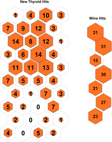
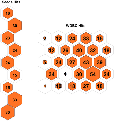
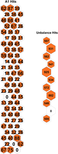
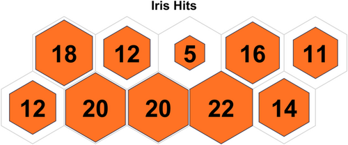
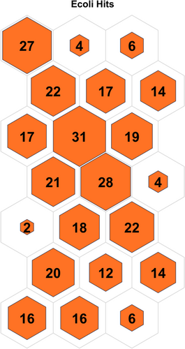
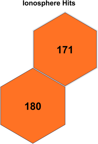
Table 3 displays the configuration used in the code executed for each data set. Table 4 displays the results obtained on all the data sets, and the contingency matrix of each data set is displayed below. Figures 5-11 display the SOM maps (microclusters of each data set), showing the hits on the respective neurons (microclusters) obtained after applying them to D_n. One of the notable points about the current work is that none of the features or attributes is neglected in any of the experiments. Nidheesh et al. work on clustering involves data sets like the Iris, New Thyroid, Wine, Breast Cancer, and Seed data sets using k-means in addition to other algorithms, including SOM, where it uses a map of 5 × 5 dimensions uniformly on all the data sets and then applies a cut tree to finally cluster the data into an actual number of clusters [15]. Their results (k-means++ and SOM) are compared with the current work, and better results are achieved. Franti et al. have used the k-means algorithm on the benchmark synthetic data sets, and a few of them, like, A1 and unbalance, have been experimented with in the current work and achieved high ARI on the same [18].

Table 3. Details of the experiments performed.

Data set	Optimal dimension of SOM for data set (D_n)	Dimension of SOM for respective weight matrix	Max epoch limit for (D_n)	Max epoch limit for weight matrix	Optimized score strategy
Iris	5 × 2	3 × 1	500	100	Calinski–Harabasz
New Thyroid	4 × 10	3 × 1	500	100	Silhouette
Wine	1 × 7	3 × 1	1350	100	Calinski–Harabasz
Seeds	1 × 9	3 × 1	500	100	Calinski–Harabasz
WDBC	5 × 5	2 × 1	500	100	Calinski–Harabasz
A1	3 × 25	20 × 1	1000	100	Calinski–Harabasz
Unbalance	1 × 11	8 × 1	500	100	Calinski–Harabasz
Dermatology	5 × 6	6 × 1	1000	500	Silhouette
Ecoli	3 × 7	8 × 1	1000	500	Silhouette
Ionosphere	1 × 2	1 × 2	1000	500	Silhouette

Abbreviation: WDBC, Wisconsin diagnostic breast cancer.

Table 4. ARI obtained on the data sets.

Algorithm	Iris	New Thyroid	Wine	Seeds	WDBC	Unbalance	A1	Dermatology	Ecoli	Iono	Reference
	Data set
HSOM (proposed approach)	0.7173	0.8041	0.9134	0.7781	0.7543	0.8755	0.8907	0.7543	0.5013	0.1728
DKM++	0.716	0.628	0.869	0.705	0.73	–	–	–	–	–	[12]
k-Means++	0.668	0.612	0.839	0.699	0.73	–	–	–	–	–	[12]
DKM	0.716	0.628	0.837	0.705	0.73	–	–	–	–	–	[12]
k-Means	0.647	0.622	0.863	0.705	0.73	0.64	0.82	–	–	–	[12]
SOM	0.683	0.568	0.739	0.586	0.388	–	–	–	–	–	[12]
NeuralGas	0.716	0.628	0.861	0.7	0.731	–	–	–	–	–	[12]
HC-single	0.558	0.075	0.004	0	0.005	–	–	–	–	–	[12]
HC-centroid	0.564	0.128	0	0.507	0.005	–	–	–	–	–	[12]
HC-comp	0.706	0.518	0.81	0.566	0.34	–	–	–	–	–	[12]
HC-average	0.72	0.111	0.004	0.725	0.005	–	–	–	–	–	[12]
PAM	0.745	0.628	0.726	0.706	0.755	–	–	–	–	–	[12]
SC	0.565	0.439	0.887	0.621	0.386	–	–	–	–	–	[12]
k-Means	–	–	–	–	–	–	–	0.3542	–	–	[28]
LI_BIFCM	–	–	–	–	–	–	–	0.7447	–	–	[28]
DBSCAN	–	–	–	–	–	–	–	0.4106	–	–	[28]
DP-chDPC	–	–	–	–	–	–	–	–	0.3620	–	[29]
DSCE	–	–	–	–	–	–	–	–	–	0.163 ± 0.014	[30]

Abbreviations: ARI, adjusted randomized index; DBSCAN, density-based spatial clustering of applications with noise; DKM, differentiable k-means clustering; DP-chDPC, density peak clustering algorithm for differential privacy protection; DSCE, dual-similarity clustering ensemble method; HC, Hierarchical clustering; HSOM, hierarchical self-organizing map; LI_BIFCM, local information bi-directional fuzzy C-means clustering; PAM, partition around medoids; SC, spectral clustering; SOM, self-organizing map; WDBC, Wisconsin diagnostic breast cancer.

5 CONCLUSIONS AND FUTURE SCOPE

From the experiments performed and the results obtained (Tables 3 and 4), it is revealed that the ARI obtained on the given data sets is better than other approaches [15, 18, 28-30]. The other observed phenomenon is that whenever clustering is performed using the SOM, the most optimum 2D configuration would be preferable by considering the ST or CH score to obtain optimized results because the WM of the SOM is also very meaningful. The future scope of this work is to apply it to gene expression data sets, as it is one of the major applications of data clustering apart from data sets from other domains. Further, the proposed technique will give better results if it is applied to selected attributes (features) of the particular data set, as most of the research data available on the web shows extensive use of feature reduction techniques and the elimination of noisy data to obtain better results.

AUTHOR CONTRIBUTIONS

Kshitij Tripathi: Conceptualization, methodology, data preprocessing, evaluation, result analysis, editing, writing, figures and drawing, and visualization.

ACKNOWLEDGMENTS

None.

CONFLICT OF INTEREST STATEMENT

The author declares no conflict of interest.

ETHICS STATEMENT

All the data sets used in this article are publicly available on the UCI repository.

INFORMED CONSENT

Not applicable.

Open Research

DATA AVAILABILITY STATEMENT

Data that support the findings of this study are available on request from the corresponding author. Data is openly available in a public repository that issues data sets with DOIs.

REFERENCES

1Tripathi K, Vyas RG, Gupta AK. The classification of data A novel artificial neural network (ANN) approach through exhaustive validation and weight initialization. Int J Comput Sci Eng. 2018; 6(5): 241–254. https://doi.org/10.26438/ijcse/v6i5.241254
10.26438/ijcse/v6i5.241254
Google Scholar
2Tripathi K, Khan FA, Khanday AMUD, Nisa KUL. The classification of medical and botanical data through majority voting using artificial neural network. Int J Inf Technol. 2023; 15(6): 3271–3283. https://doi.org/10.1007/s41870-023-01361-0
10.1007/s41870-023-01361-0
Google Scholar
3Tripathi K, Vyas RG, Gupta AK. Document classification using artificial neural network. Asian J Comput Sci Technol. 2019; 8(2): 55–58. https://doi.org/10.51983/ajcst-2019.8.2.2140
10.51983/ajcst-2019.8.2.2140
Google Scholar
4Kumar S. Neural networks: a classroom approach. New Delhi: Tata McGraw-Hill Education; 2004.
Google Scholar
5Han J, Pei J, Kamber M. Data mining: concepts and techniques. Waltham, MA: Morgan Kaufmann Publishers, Elsevier; 2011.
Google Scholar
6Rousseeuw PJ. Silhouettes: a graphical aid to the interpretation and validation of cluster analysis. J Comput Appl Math. 1987; 20(1): 53–65. https://doi.org/10.1016/0377-0427(87);90125-7
10.1016/0377-0427(87)90125-7
Web of Science® Google Scholar
7Calinski T, Harabasz J. A dendrite method for cluster analysis. Commun Stat—Theory Methods. 1974; 3: 1–27. https://doi.org/10.1080/03610927408827101
10.1080/03610927408827101
Google Scholar
8Kohonen T. The self-organizing map. Proc IEEE. 1990; 78(9): 1464–1480. https://doi.org/10.1109/5.58325
10.1109/5.58325
Web of Science® Google Scholar
9Kohonen T. Self-organized formation of topologically correct feature maps. Biol Cybern. 1982; 43(1): 59–69. https://doi.org/10.1007/BF00337288
10.1007/BF00337288
Web of Science® Google Scholar
10Kohonen T. Analysis of a simple self-organizing process. Biol Cybern. 1982; 44(2): 135–140. https://doi.org/10.1007/BF00317973
10.1007/BF00317973
Web of Science® Google Scholar
11Lampinen J, Oja E. Clustering properties of hierarchical self-organizing maps. J Math Imaging Vision. 1992; 2(2): 261–272. https://doi.org/10.1007/BF00118594
10.1007/BF00118594
Google Scholar
12Wu S, Chow TWS. Self-organizing-map based clustering using a local clustering validity index. Neural Process Lett. 2003; 17(3): 253–271. https://doi.org/10.1023/A:1026083612746
10.1023/A:1026083612746
Web of Science® Google Scholar
13Drigas AS, Vrettaros J. Using the self-organizing map (SOM) algorithm, as a prototype E-content retrieval tool. In: Proceedings of the International Conference on Computational Science and Its Applications, Part II, Lecture Notes in Computer Science, Vol. 5073, Springer; 2008. p. 14–23.
Google Scholar
14Argyrou A. Clustering hierarchical data using self-organizing map: a graph–theoretical approach. In: Proceedings of the 7th International Workshop on Advances in Self-Organizing Maps, Lecture Notes in Computer Science, Vol. 5629, Springer; 2009. p. 19–27. https://doi.org/10.1007/978-3-642-02397-2_3
10.1007/978-3-642-02397-2_3
Google Scholar
15Nidheesh N, Abdul Nazeer KA, Ameer PM. An enhanced deterministic K-means clustering algorithm for cancer subtype prediction from gene expression data. Comput Biol Med. 2017; 91: 213–221. https://doi.org/10.1016/j.compbiomed.2017.10.014
10.1016/j.compbiomed.2017.10.014
CAS PubMed Web of Science® Google Scholar
16Ambroise C, Govaert G. Constrained clustering and Kohonen self-organizing maps. J Classif. 1996; 13(2): 299–313. https://doi.org/10.1007/BF01246104
10.1007/BF01246104
Web of Science® Google Scholar
17Jain AK. Data clustering: 50 years beyond K-means. Pattern Recognit Lett. 2010; 31(8): 651–666. https://doi.org/10.1016/j.patrec.2009.09.011
10.1016/j.patrec.2009.09.011
Web of Science® Google Scholar
18Fränti P, Sieranoja S. K means properties on six clustering benchmark datasets. Appl Intell. 2018; 48: 4743–4759. https://doi.org/10.1007/s10489-018-1238-7
10.1007/s10489-018-1238-7
Web of Science® Google Scholar
19Ray SS, Agrawal S, Ghosh S. Decision theoretic rough set-based neighborhood for self-organizing map. SN Comput Sci. 2021; 2(2): 102. https://doi.org/10.1007/s42979-021-00490-2
10.1007/s42979-021-00490-2
Google Scholar
20Nguyen HN, Tran NN, Hoang TH, Cao VL. Denoising latent representation with SOMs for unsupervised IoT malware detection. SN Comput Sci. 2022; 3(6): 474. https://doi.org/10.1007/s42979-022-01344-1
10.1007/s42979-022-01344-1
Google Scholar
21Ripan RC, Sarker IH, Hossain SMM, Anwar MM, Nowrozy R, Hoque MM, et al. A data-driven heart disease prediction model through K-means clustering-based anomaly detection. SN Comput Sci. 2021; 2(2): 112. https://doi.org/10.1007/s42979-021-00518-7
10.1007/s42979-021-00518-7
Google Scholar
22Tarekegn AN, Michalak K, Giacobini M. Cross-validation approach to evaluate clustering algorithms: an experimental study using multi-label datasets. SN Comput Sci. 2020; 1(5): 263. https://doi.org/10.1007/s42979-020-00283-z
10.1007/s42979-020-00283-z
Google Scholar
23Chen H, Ge M, Xue Y. Clustering algorithm of density difference optimized by mixed teaching and learning. SN Comput Sci. 2020; 1(3): 172. https://doi.org/10.1007/s42979-020-00183-2
10.1007/s42979-020-00183-2
Google Scholar
24Townsley SK, Basu D, Vora J, Wun T, Chuah CN, Shankar PRV. Predicting venous thromboembolism (VTE) risk in cancer patients using machine learning. Health Care Sci. 2023; 2(4): 205–222. https://doi.org/10.1002/hcs2.55
10.1002/hcs2.55
Google Scholar
25Wang X, Zhang D. Choices of medical institutions and associated factors in older patients with multimorbidity in stabilization period in China: a study based on logistic regression and decision tree model. Health Care Sci. 2023; 2(6): 359–369. https://doi.org/10.1002/hcs2.73
10.1002/hcs2.73
Google Scholar
26Kelly M, Longjohn R, Nottingham K. The UCI Machine Learning Repository; 2013. Available from: https://archive.ics.uci.edu
Google Scholar
27Hubert L, Arabie P. Comparing partitions. J Classif. 1985; 2: 193–218. https://doi.org/10.1007/BF01908075
10.1007/BF01908075
Web of Science® Google Scholar
28Ren C, Sun L. A bi-directional fuzzy C-means clustering ensemble algorithm considering local information. Int J Comput Intell Syst. 2021; 14(1): 171. https://doi.org/10.1007/s44196-021-00014-z
10.1007/s44196-021-00014-z
Web of Science® Google Scholar
29Chen H, Mei K, Zhou Y, Wang N, Tang M, Cai G. A density peaking clustering algorithm for differential privacy preservation. IEEE Access. 2023; 11: 54240–54253. https://doi.org/10.1109/ACCESS.2023.3281652
10.1109/ACCESS.2023.3281652
Web of Science® Google Scholar
30Alqurashi T, Wang W. Clustering ensemble method. Int J Mach Learn Cyber. 2019; 10: 1227–1246. https://doi.org/10.1007/s13042-017-0756-7
10.1007/s13042-017-0756-7
Web of Science® Google Scholar

Volume3, Issue2

April 2024

Pages 88-100

This article also appears in:

2024 Top Viewed Health Care Science Articles

The novel hierarchical clustering approach using self-organizing map with optimum dimension selection