Under the effect of various hydrodynamic forcings, the morphology of the coastal zone and more particularly the intertidal zone is subject to short-term variations. Capable of autonomous continuous recording, video camera systems offer a good opportunity to capture these short-term morphological variations. Extracting a topography of the intertidal zone from these videos involves detecting successive shorelines on the foreshore during a tidal cycle by assigning them an altitude. Detecting this shoreline is therefore a key stage. Here, considering the shoreline as the boundary between a moving zone (wave breaking) and a supposedly stable zone, we propose a method based on ‘variance images’ (in reality, calculated as the median for 5 min video of the standard deviations on radiometry of each pixel over 10 s intervals). The method was evaluated at four sites with different geo-morphological characteristics, different camera installations and with a wide range of weather conditions (including stormy ones). Of the 111 randomly selected images, 73% of the shorelines were correctly detected (reaching 95% for the Ruscumunoc site). These raw results could be further improved by adding a filtering step or by optimising the installation (avoiding mast vibrations, pruning vegetation, etc.). The Digital Elevation Models (DEMs) generated potentially on a daily basis over the intertidal zone will make it possible to study topographic variations under different conditions (reconstructive regime, impact of an extreme event, etc.).

1 INTRODUCTION

Coastal environments, and particularly beaches, are exposed to multiple, highly dynamic forces (natural and anthropogenic) and therefore are prone to rapid changes in their morphology: beach erosion/nourishment, creation of a berm or beach cusps, etc. Topographic monitoring of beaches is traditionally carried out using GNSS RTK, either via cross-shore profiles (e.g. Bertin et al., 2022; Suanez et al., 2023) or by equipping a vehicle to cover the entire surface of the beach (e.g. Castelle et al., 2020; Morton et al., 1993). Spatialised monitoring has been facilitated by very high-resolution remote sensing methods such as Terrestrial Laser Scanning (TLS - e.g. Bertin et al., 2022; Jaud et al., 2017; Lapietra et al., 2022) or unmanned aerial vehicle (UAV) photogrammetry (e.g. Casella et al., 2016; Jaud et al., 2019; Long et al., 2016). However, these methods do not allow both daily and long-term monitoring.

Implemented since the 1990s (Holland et al., 1997; Holman et al., 1993), video imaging systems have become classic tools for coastal monitoring. Commercial systems (e.g. ARGUS - Holman et al., 1993 - or Spectur® CoastalComs) and open source systems (e.g. SIRENA® by Imedea & Socid - Nieto et al., 2010) have been developed. More recently, studies have also been conducted to take advantage of existing systems (ex. SurfCam – Andriolo, Sánchez-García, & Taborda, 2019; Bracs et al., 2016). In all cases, camera observation remains an inexpensive way of providing continuous (high-frequency) monitoring with very little operator involvement, and for a wide variety of possible applications.

Different products (with different degrees of processing and analysis) can be extracted from the video, and the spatial and temporal sampling strategy depending on each specific issue (Holman & Stanley, 2007). Simple snapshots extracted from the video can be useful for coastal management, through the assessment of visitor numbers or the creation of monitoring indicators (Arnberger, Haider, & Brandenburg, 2005; Guillén et al., 2008; Van Koningsveld et al., 2007).

A ‘standard’ by-product is a time-averaged image. For Argus systems, this image (originally generated every hour) is called ‘Timex’ (for time exposure) and corresponds to the average of frames collected at 1 or 2 Hz over a 10-minute period of sampling (Holman & Stanley, 2007). From the same set of image samples, “variance images” are also generated from the variance of image intensities (Holman & Stanley, 2007). ‘Stacks’ are another standard product derived from these videos. Time-stacks are a time–space representation designed to maintain full temporal resolution (e.g. 2 Hz for the Argus system), but only along one (or more) transect, generally cross-shore, observed over a period of time (Holman & Stanley, 2007). We also find these representations of cross-shore profiles over time applied to 10-minute Timex average images (‘TimexStack’) or variance images (‘VarStack’)(Andriolo, 2019).

Working with 1D profiles optimises processing times. In addition, because ‘stacks’ can offer very high temporal resolution, they are preferentially used for hydrodynamic issues, as extracting nearshore wave properties (e.g. Almar et al., 2009; Colvin, Lazarus, & Splitt, 2020; Osorio et al., 2019; Ramesh et al., 2022) and estimating the position of the breakpoint and the extent of shoaling, surf and swash zone (e.g. Andriolo, 2019). These time–space representations are also used to calculate bathymetry by inversion based on wave observation (e.g. Brodie et al., 2018; Stockdon & Holman, 2000). Some studies provide longshore information by reproducing this stack analysis on several cross-shore profiles (Andriolo, 2019; Bergsma et al., 2016; Jóia Santos, Andriolo, & Ferreira, 2020; Nuyts et al., 2024). On the other hand, time-averaged products (such as Timex or variance images) allow the full spatial resolution of longshore data to be exploited. In addition, averaging these data removes high-frequency signals (particularly waves) and allows each image to be associated with an average water level. Knowing the water level and, from the videos, the position of the shoreline (i.e. water/beach interface) over time, it is possible to reconstruct the topography of the intertidal zone at each tidal cycle (e.g. Aarninkhof et al., 2003; Almar et al., 2012; Montes et al., 2023; Soloy et al., 2021).

Many studies have already looked at shoreline detection using video imagery. Nuyts et al. (2024) studied the impact of the temporal sampling strategy to produce an averaged image for shoreline detection. Almar et al. (2012) have already shown that using images averaged over a shorter period (30 s) improves the accuracy of shoreline detection. Furthermore, different approaches are implemented to identify the shoreline position on these averaged images. Manual digitisation (e.g. Chang et al., 2019) is of course, highly time-consuming and not sustainable for dense long-term data series. Shore Line Intensity Maximum (SLIM) was proposed by Plant & Holman (1997) for greyscale cameras to localised the maximum wave breaking. Inherited from the SLIM method, several approaches are based on radiometric variations in the different bands of Red-Green-Blue (RGB) or Hue-Saturation-Value (HSV) images to detect the limit between water and sand or between the dry and wet sands. For example, the CCD (Colour Channel Divergence) model of Turner et al. (2001), the PIC (Pixel Intensity Clustering) method (based on HSV intensity difference) proposed in Aarninkhof et al. (2003), the ANN (Artificial Neural Network) model of Kingston (2003), or the Minimum Shoreline Variability (MSV) developed by Almar et al. (2012). These approaches have been made more robust by optimised segmentation methods, as semantic segmentation of the Shoreline Detection Model (SDM) (Valentini et al., 2017) or as edge detection via the Physical and Statistical Detection Model (PSDM) (Osorio, Medina, & Gonzalez, 2012), which combines different edge/shoreline-detection algorithms and physical and statistical criteria. However, these radiometry-based methods are highly dependent on lighting conditions (and therefore sensitive over the long term to variations in weather conditions) and require site-specific parameterisation depending on the colour of the beach (sand, pebbles, the shadow of a cliff, etc.).

New approaches exploiting the capabilities of Artificial Intelligence and Deep Learning are also emerging (e.g. polynomial radial basis function [RBF] neural network used by Rigos et al., 2016 – or the deep learning algorithm Mask R-CNN used by Soloy et al., 2021). These methods appear to have great potential, particularly in terms of transferability to all types of environments, but they require the algorithm to be trained, which can be very time-consuming in order to be effective.

Some studies combine radiometric information with variance information. In river streams, Stumpf et al. (2016) used a combination of radiometric thresholding and variance of the mean brightness for water surface detection. The study by Simarro et al. (2015) looked at the possibility of using variance images (corresponding to the 10 min radiometry standard deviation of 1 snapshot per second) in coastal zones, but no shoreline extraction results were presented. Vousdoukas et al. (2011) combined variance images (over a time interval of 5 to 30 min) and Neural Network for shoreline detection. Andriolo (2019) exploited the pixel intensity variation in the different bands to automatically retrieve the nearshore wave transformation domains.

The aim of the present study is to implement a simple and robust method fully based on variance images for extracting the shoreline from nearshore videos. This approach is being evaluated independently of subsequent filtering modules, over several survey sessions lasting several months, with different types of meteorological and hydrodynamic conditions, in a macrotidal context, with different acquisition configurations (camera on a mast or on a cliff, with different orientations) and on different types of beach (pebble or sand, dissipative, intermediate or reflective).

2 STUDY AREAS AND DATA ACQUISITION

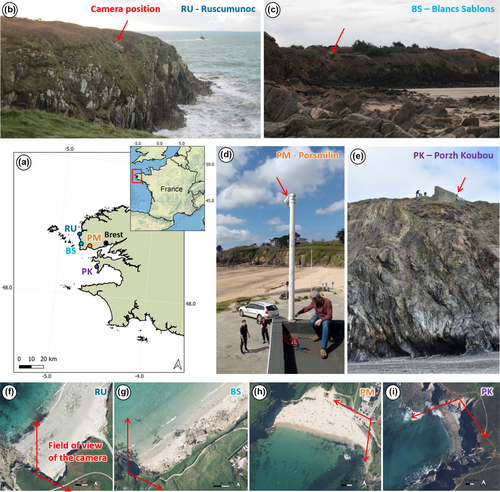
In order to assess the robustness of the method proposed in this study, we used various datasets of video acquired at four sites in Finistère (Brittany, France), but with distinct morphological characteristics: Ruscumunoc (RU), Blancs Sablons (BS), Porsmilin (PM) and Porzh Koubou (PK) (Figure 1). These four sites are subject to a macro-tidal regime and a temperate oceanic climate where winters can be stormy (e.g. Bertin et al., 2022; Stéphan et al., 2019). The cameras at Ruscumunoc and Blancs Sablons were installed to record erosion events on the cliff face and not to observe the beach. Their angle of view is therefore not optimised for this purpose, but the images are nonetheless usable for this study. Figure 1 provides an overview for comparing these different sites. As the camera models, installation and settings also vary from one site to another, Table 1 summarises this information.

Details are in the caption following the image — **FIGURE 1**
Open in figure viewer PowerPoint

a) Map of the four study areas along the western coast of Brittany, France. b) c) d) e) Environment for installing the camera in Ruscumunoc (b), Blancs Sablons (c), Porsmilin (d) and Porzh Koubou (e). f) g) h) i) Approximate field of view of the camera represented on ortho-images (source: BD-ortho IGN®) in Ruscumunoc (f), Blancs Sablons (g), Porsmilin (h) and Porzh Koubou (i).

TABLE 1. Camera characteristics and setup in each study area.

	Ruscumunoc (RU)	Blancs Sablons (BS)	Porsmilin (PM)	Porzh Koubou (PK)
Video camera model	Axis P1355-E	Axis P1355-E	Axis P1377-LE	Axis P1377-LE
Power supply	Solar panel	Solar panel	Mains supply	Solar panel
Image resolution	1920 × 1,080	1920 × 1,080	2,592 × 1944	2,592 × 1944
Sampling frequency	4 fps*	4 fps	5 fps	5 fps
Camera support	Installed on a concrete base	Installed on a concrete base	Installed on a 3 m-high mast	Installed on a concrete base
Camera orientation	NE	NE	SW	S
Period of monitoring	Nov. 2015 – Apr. 2016	Jan. 2016 – Apr. 2016	Nov. 2021 - to present	Jan. 2020 – to present
Acquisition setup	Acquisitions around high tide (HT-2 h to HT + 2 h) + 15 min at low tide (daytime only)	Acquisitions around high tide (HT-2 h to HT + 2 h) + 15 min at low tide (daytime only)	Acquisitions of 10 min every 20 min (day and night)	Acquisition 25 min every 30 min (daytime only)
Observed area	Intermediate sandy beach (with rocks and cobbles on the upper part) and cliff	Dissipative sandy beach (with rocks and cobbles on the upper part) and cliff	Intermediate sandy beach	Wave-cut platform, reflective gravel beach and cliff

* fps: frame per second.

2.1 Ruscumunoc

Facing north-west (Figure 1f), Ruscumunoc is a site of cliffs at the foot of which nestles a sandy beach visible only at neap or low tide. This beach is of the intermediate type (according to the beach state classification in Wright & Short, 1984), with an average beach face gradient of 0.06 over the study period. Sometimes, rocks or cobble patches may appear on the beach. As mentioned, the purpose of this camera monitoring was to observe the dynamics of the cliff face and it only lasted one winter, from November 2015 to April 2016. The camera was installed on a concrete support, nearly at the top of the cliff (Figure 1b), a remnant of the Atlantic Wall from the Second World War (WW2). In order to limit storage space, the sampling frequency of the video is parameterised to four frames per second (fps) and recording was programmed only during daytime, continuously for 4 hours around the peak of high tide (HT), when marine forces were most likely to generate gravity movement, and 15 minutes at low tide.

2.2 Blancs Sablons

Blancs Sablons is a dissipative, north-west-facing beach divided into three beach compartments separated by rocky spurs (Dehouck, 2006). The average beach gradient of 0.02 is nearly homogeneous cross-shore. The beach is constrained to the south and north by rocky cliffs. The two northern compartments are closed off from the backshore by a dune belt, while the southern compartment is closed off by a ~ 10 m-high cliff. In this southern compartment, rocks or cobble patches may sometimes appear on the upper part of the beach. As with Ruscumunoc, it was the cliff bordering this southern compartment that was originally the focus of the camera monitoring (Figure 1g). The monitoring only covered a few winter months, from January 2016 to April 2016, with recording scheduled only during the daytime, at 4 fps, continuously for 4 hours around the peak of high tide and 15 minutes at low tide. The camera was installed on a concrete support, in the opening of a blockhouse left over from the Atlantic Wall (WW2), at the top of the south cliff (Figure 1c).

2.3 Porsmilin

Located at the entrance to the Bay of Brest, Porsmilin is a sandy beach at the bottom of a cove, bordered by cliffs 10–15 m high to the west and east and a small dune (~1 to 2 m high) to the north (Figure 1a and h). This beach, which has been monitored since 2003 using various techniques (cross-shore profiles, terrestrial Lidar, photogrammetry, bathymetric sounder) has already been described many times in the literature (e.g. Bertin et al., 2022; Caulet, 2018; Dehouck, 2006; Jaud et al., 2019). This monitoring is carried out as part of the SNO-DYNALIT (https://www.dynalit.fr/) national observation service from ILICO French Research Infrastructure. Porsmilin beach is of the intermediate type, with an average beach slope ranging from 0.02–0.04 on the shoreface to 0.04–0.08 on the intertidal and upper beach. Patches of cobbles may appear intermittently, mainly at the top of the beach and at the top of the foreshore. Dark deposits of peat also sometimes appear at the bottom of the foreshore.

An initial video camera was installed at Porsmilin in September 2014. However, as this article does not aim to generate a series of data, we will only look at the data collected by the Axis P1377-LE camera installed in November 2021 (replacing the previous camera). Facing south-west, this camera captures virtually the entire beach. It is fixed to the top of a 3 m high mast, itself fixed to a 3.5 m high building, to the east of the access car park (Figure 1d and h). The camera collects 10 min of video every 20 min, with a sampling frequency of 5 fps.

2.4 Porzh Koubou

The Porzh Koubou site is located further south, in the Crozon peninsula. The rocky cliffs of Porzh Koubou, around 40 m high, are studied as part of the national SNO-DYNALIT observation service (surveys of the cliff face are carried out twice a year). In the Porzh Koubou cove (Figure 1i), at the foot of the cliffs, there is a gravel beach, continuing onto the foreshore with a rocky flat on which sand may be present intermittently. The gravel beach is reflexive and sometimes forms beach cusps. The camera is installed here to the north of the area, on the side of a concrete wall at the top of the cliff (Figure 1e), the remains of a pebble loading station (formerly mined). The camera is set up to capture 25 minutes of video (5 fps) every 30 minutes, during daytime only.

3 METHODS

The general principle of the method is that, from a video, knowing the calibration parameters (internal and external) of the camera, it is possible to find the XY position of each pixel in map coordinates. Knowing the altitude of a water level at a given moment, by extracting the shoreline, we can obtain the XYZ map coordinates of all the pixels located on this shoreline. So, once the successive shorelines have been extracted throughout a tidal cycle, and a water level (from a pressure sensor or a model) and therefore an altitude have been associated with them, a Digital Elevation Model (DEM) of the foreshore can be reconstructed (Figure 2). The originality of this study lies in the shoreline detection and extraction method, so the other stages of the procedure are not described in much detail as they are similar to what is described in the literature (e.g. Aarninkhof et al., 2003; Vousdoukas et al., 2011).

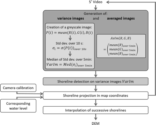
For camera calibration, the internal orientation parameters are computed from a series of images of a checkerboard, viewed from different positions and in different orientations. The external orientation parameters are computed from Ground Control Points (GCPs), manually identifying a target moved by an operator in the imaged zone and measured by a Real-Time Kinematic Global Navigation Satellite System – RTK GNSS – with centimetric accuracy.

For shoreline detection, the dataset consists of a series of 5-minute videos (with the highest temporal resolution, i.e. at 4 or 5 fps depending on the site). As suggested in the study by Simarro et al. (2015), the idea is to take advantage of the ‘dynamic’ aspect of video. In a time series of images, movement is expressed by a change in the radiometry of a given pixel. Although generally referred to as ‘variance’ (Andriolo, 2019; Simarro et al., 2015), it is actually the temporal standard deviation of the radiometry of the pixels that is calculated. As the surf zone is constantly dynamic, the shoreline is defined as “the most shoreward maximum corresponding to the swash zone” (e.g. Andriolo, 2019; Simarro et al., 2015; Vousdoukas et al., 2011).

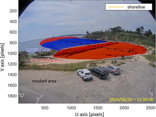
In our approach, to avoid disturbance from movements outside the intertidal zone (people on the upper beach, vehicles, birds, insects, vegetation moving in the wind), a Region Of Interest (ROI) is manually defined once for each study site (Figure 3). This ROI must encompass all areas of the image where the shoreline can be located. The cross-shore axis is also roughly defined once for each study area (Figure 3).

As Almar et al. (2012) did with the Minimum Shoreline Variability (MSV) approach for colour ratios, we will work over short periods (5 min) to avoid the effects of the tide and maintain high spatial resolution. The calculation is performed in the following steps (Figure 2):

For each pixel of each frame, calculation of the average of the R, G and B bands to create a greyscale image.
Calculation of temporal standard deviations on radiometry of each pixel over 10 s intervals. The duration of 10 s is set empirically and corresponds to an order of magnitude of the wave period.
For each pixel, for 5 min of video, calculation of the median of the standard deviations to create the “variance image” VarIm. The duration of 5 min offers a good compromise between a duration short enough for the tidal effect to be considered negligible and long enough to capture only repeated movements in the same area while filtering out sporadic movements.
The ROI of the greyscale VarIm is converted into a binary image, and classified into moving areas (corresponding to the swash zone) and stable areas (Figure 3) using the Otsu method for grey-level histograms (Otsu, 1979).

For this classification, the “variance” values VarIm are separated into L intervals [I₁, I₂, …, I_L], with [c₁, c₂, …, c_L] as their respective centres. The number of pixels in VarIm whose value lies within the interval I_i is called n_i. The total number of pixels in the image is given by the formula N = n₁ + n₂ + … + n_L and the fraction of pixels in each interval is expressed as p_i = n_i/N.

To determine the optimum threshold, Otsu (1979) suggests considering the between-class variance (Equation 1):

{\sigma}_B^2(k)=\frac{{\left[{\mu}_T\omega (k)-\mu (k)\right]}^2}{\omega (k)\left[1-\omega (k)\right]}\ where\ k\ \epsilon\ \left[1,L\right]

(Eq 1)

\mathrm{with}\ \omega (k)=\sum \limits_{i=1}^k{p}_i,\mathrm{the}\ \mathrm{probability}\ \mathrm{of}\ \mathrm{class}\ \mathrm{occurrence}

(Eq 2)

\mu (k)=\sum \limits_{i=1}^k{c}_i{p}_i,\mathrm{the}\ \mathrm{class}\ \mathrm{mean}\ \mathrm{level}

(Eq 3)

{\mu}_T=\mu (L)=\sum \limits_{i=1}^L{c}_i{p}_i,\mathrm{the}\ \mathrm{total}\ \mathrm{mean}\ \mathrm{level}\ \mathrm{of}\ \mathrm{the}\ \mathrm{original}\ \mathrm{picture}.

(Eq 4)

The optimal threshold k* (Equation 5) that maximises the between-class variance and minimises the within-class variance, is such that:

{\sigma}_B^2\left({k}^{\ast}\right)=\underset{1\le k\le L}{\max }{\sigma}_B^2(k)

(Eq 5)

To extract the shoreline, the most ‘shoreward’ part of the moving zone is isolated, considering the most onshore pixel between the moving zone and the fixed zone along the cross-shore direction defined previously by the profile (Figure 3). To take account of local variations in the direction of the shoreline (presence of beach cusps, for example), a tolerance of +/−20° in relation to the longshore axis (considered to be perpendicular to the cross-shore axis defined manually for each site) is allowed.

In addition to the variance image, an RGB image averaged over 5 minutes (AvIm – Figure 2) is also generated. This averaged image is of no use when detecting the shoreline, but it does provide a visual control when displaying the detected shoreline (Figure 4).

In this approach, the series of images is never projected in map coordinates. The calibration parameters (internal and external) are used to project only the shoreline pixels, which considerably reduces processing times. In our case, for a 5-minute video, generating VarIm variance images and AvIm RGB averages takes around 24 seconds/video (parallelised over 10 cores) and shoreline detection takes around 2 seconds/video. In this study, apart from the definition of the ROI and the cross-shore direction specific to each site, the detection algorithm remains rigorously identical between the different sites.

4 RESULTS

4.1 Qualitative validation

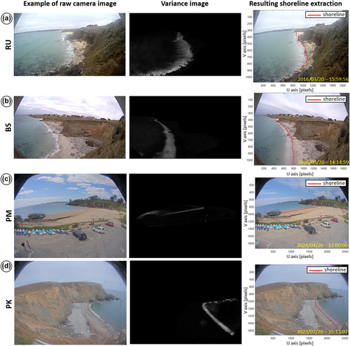
In this study, the quality of detection is assessed by expert eyes, for each image, by classifying according to three categories:

valid detection (the shoreline can be used as is) (Figure 4);
intermediate quality detection (the shoreline is not usable as it stands, but could become usable by redefining the ROI or filtering the data) (Figure 5a and b)
invalid detection (the pixels detected do not correspond or do not completely correspond to the shoreline) (Figure 5c and d).

In order to cover the widest range of configurations, in terms of tide level, luminosity, weather conditions (rain, wind, fog), wave conditions, site frequentation, etc., without however creating a bias in the representativeness of certain conditions, the images are chosen randomly throughout each monitoring period. Given the short monitoring periods at Ruscumunoc and Blancs Sablons, 1 image is assessed every 5 days (only ‘winter’ conditions are represented at these sites). For monitoring at Porsmilin and Porzh Koubou, 1 image is taken every 10 days. As a result, the number of shorelines assessed differs from site to site (Table 2).

TABLE 2. Results of the quality assessment of the shoreline extraction.

	RU	BS	PM	PK
Number of images assessed	21	17	38	35
Number of valid detections	20	7	27	27
Number of intermediate quality detections	0	1	2	7
Number of invalid detections	1	9	9	1
% of valid detections	95%	41%	71%	77%

In total, a sample of 111 images from all the sites were evaluated, with a valid detection rate of 73%. Table 2 shows the results of this evaluation site by site. At Ruscumunoc, 95% of valid detections were obtained, corresponding to a single bad detection despite very unfavourable weather conditions on certain days (Figure 6). The Blancs Sablons site had the lowest success rate, with only 41% of valid detections. The Porsmilin and Pozh Koubou sites had a valid detection rate close to the average, with 71% and 77% respectively.

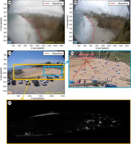
There is a disparity in success rates depending on the site. The Ruscumunoc and Blancs Sablons sites are only monitored in winter (a period that is, in theory, more unfavourable), but this is not a sufficient explanation for the disparities, as Ruscumunoc has the best success rate (95%) while Blancs Sablons has the lowest (41%). At Blancs Sablons, as the beach is dissipative, the waves begin to dissipate their energy (wave breaking) away from the shoreline. Under energetic conditions, the foam associated with this breaking zone covers a large cross-shore area of the image, implying few colour variations and therefore a very homogeneous variance throughout the foam-covered zone. In the absence of a marked peak of maximum variance, shoreline detection is unlikely to be effective (Figure 5d). In calm conditions, there is less foam, the radiometry changes of the same pixel are more marked and shoreline detection is more effective (Figure 4b). Consequently, on a dissipative beach, the effectiveness of the method depends on the weather conditions.

At Porsmilin, tourist displacements on the beach is sometimes a source of false detections. However, the most frequent case of false detections is caused by camera movement due to mast vibrations. These vibrations make ‘fixed’ elements appear to be ‘moving’ in the variance image, leading to invalid (or intermediate) detections (Figure 5b and c). At the other sites, where the camera is mounted directly on a concrete support, this problem was not detected. The detection rate at Porsmilin could therefore be improved by rethinking the way the camera is installed.

At Porzh Koubou, 20% of the detections were of ‘intermediate quality’, mainly due to a bramble that had grown in front of the camera and which became agitated when there was wind, locally creating a variance signal stronger than that of the surf (Figure 5a). Here again, by regularly clearing the site, the rate of valid detections could be improved.

In all cases, adding post-processing steps (such as filtering or smoothing) could help to improve these results. But their parameters would probably be site-dependent.

4.2 Indirect quantitative validation in Porsmilin

By associating a water level with the shorelines detected, it is possible to assign them an altitude and thus project them into a cartographic reference frame (X,Y,Z). The water level visible in the images is the result of a combination of several factors: the effect of the tide (η_tide - estimated using a local tide model), the surges due to atmospheric pressure and wind (η_pressure + η_wind - measured at a nearby tide gauge) and the effect of the setup (η_setup). In the case at hand, at Porsmilin Beach, an in situ pressure sensor (located at ~16 m depth from the lowest astronomical tide) is also used to measure η_tide + η_pressure + η_wind.

The question of how to determine the wave setup is the subject of numerous studies which have proposed different methods (e.g. Bowen, Inman, & Simmons, 1968; Guza & Thornton, 1981; Holman & Sallenger, 1985; Stockdon et al., 2006). As this is not the subject of the present study, we will use an empirical model by Stockdon (Stockdon et al., 2006), in which the wave setup is parameterised on the basis of the beach slope determined from a ‘calibration profile’, measured on 2022/02/02, using RTK GNSS and the wave height and wavelength measured simultaneously by the pressure sensor.

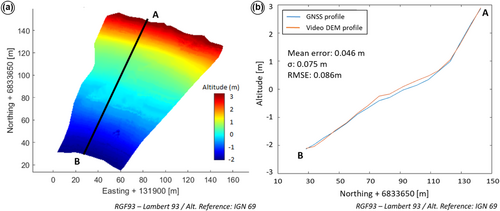
The processing chain (Figure 2) was therefore applied in its entirety to generate DEMs of the inter-tidal zone, on 2022/03/30. In this case, the DEM is the result of a linear interpolation of successive shorelines (projected in RGF93 - Lambert93 coordinates and altitudes referred to IGN69) on a regular grid with a horizontal resolution of 50 cm.

Comparison of this DEM with synchronous cross-shore profiles (measured using RTK GNSS with centimetric accuracy) indirectly validates the relevance of the shorelines extracted. Nevertheless, the reconstructed DEM is also affected by uncertainties related to the association of a water level with a shoreline and uncertainties in the projection of pixel coordinates to map coordinates. Uncertainty in the position of the shoreline encompasses the uncertainties associated with its detection on the image as well as the errors associated with its projection from image coordinates (in pixels) to map coordinates (considering the camera's internal and external parameters, the impact of resolution as a function of distance from the camera, etc.). In some cases, it may be difficult to distinguish the sources of error.

Figure 7a shows an example of reconstruction of the foreshore DEM from video and comparison with a cross-shore topographic profile on 30 March 2023. The average error is 4.6 cm and the standard deviation is 7.5 cm, which is fairly representative of the quality of our reconstructions, since over a series of 10 comparisons with GNSS RTK profiles at different times of the year, we obtained an average error of 4.4 cm and a standard deviation of 8.6 cm. Figure 7b shows that the difference between the profiles is mainly located on the foreshore area with the lowest slope. The areas with gentle slopes are those where there is the most uncertainty in detecting the shoreline. This variation in the slope of the beach also implies an overestimation of the setup (which normally decreases when the slope of the beach is lower) and therefore an overestimation of the altitudes associated with the shorelines in this area. This overestimation of the setup could explain why the profile extracted from the DEM reconstructed from the video appears above the GNSS RTK profile.

5 DISCUSSION

5.1 Limits and advantages of the method

This shoreline detection method takes advantage of the fact that the shoreline is the boundary between an area in motion (wave breaking) and an area that is assumed to be stable. The ‘variance’ (in reality, calculated as the median for 5 min video of the standard deviations of greyscale pixels over 10 s intervals) can be used to highlight this boundary.

Comparative tests between the different study sites highlight the limitations of the method. This variance-based detection approach is sensitive to camera movements. This constraint can be taken into account when installing the device, by favouring a fixed support (on the rock or on a concrete support) and/or sheltered from the wind, to avoid the vibrations of a mast. Detection of the shoreline is also affected by the movement of vegetation in the wind. This limitation can be considered when defining the ROI. Tourist traffic can also be a source of movement and therefore of false detections, although in our case we were not faced with this problem even though Porsmilin is a popular beach (Figure 6c). This may be due to the fact that, unlike surf, people's movements are not repeated in the same area and therefore do not create a peak of ‘variance’ when averaging over 5 min.

Despite these limitations, this variance-based detection approach gives very satisfactory results (on average, 73% across all sites), which are equivalent to or better than those reported in the literature. In a study comparing different methods applied to four different study sites, Plant et al. (2007) obtained detection rates ranging from 15% to 50% for SLIM, from 0% to 91% for CCD, from 24% to 78% for PIC and from 32% to 92% for ANN. Using Deep Learning methods (Mask R-CNN algorithm) applied to three gravel beach sites, Soloy et al. (2021) obtained success rates of 67.11%, 69.87% and 97.33% respectively, depending on the site (with weather conditions similar to ours). However, these methods involve a very time-consuming training phase (including labelling) and reduce the resolution of the shoreline (aliasing effect due to detection on a subsampled image). In addition, Soloy et al. (2021) mention that the neural network detection method loses effectiveness with distance from the waterline or in the presence of complex geometries (channels, ponds, baïnes, etc.). Finally, as with our variance method, the Deep Learning method has more difficulty detecting the shoreline when the beach is not very steep. But this comparison with other studies remains limited because the evaluation method varies from case to case. The results of this evaluation also depend on the variability of the acquisition conditions (weather conditions, site characteristics, testing on different sites, etc.) and on whether or not a post-processing step (e.g. filtering) is included in the detection method. To further evaluate our approach, we compared radiometric detection (based on RGB ratios) with our variance detection method on a sample of 120 images (different from the one used in part 4), acquired under various weather conditions and for different tide levels at the Porsmilin site. Over the whole of the intertidal zone (the foreshore can cover up to 140 m), the shoreline was correctly detected in 83% of cases with the variance method compared with 23% for the radiometry method (this score being lowered by numerous poor detections at the bottom of the foreshore).

Our variance-based method has the advantage of being very direct: no training phase as with Deep Learning methods and no exploration of the dataset to identify the most relevant ratio between the RGB bands and associated threshold as with radiometry-based methods. This variance-based approach is also robust to the ‘colour’ or variations in colour of the foreshore (algae deposits, presence of pebbles or not, change of substrate depending on the season or on the tide level) and lighting conditions, which is particularly advantageous for long time series where the site is likely to change. It even proves to be fairly robust to the presence of raindrops on the lens. However, these can cause local distortion of the image.

5.2 Impact of parameterisation for dissipative beaches

As detection on dissipative beaches is the most challenging, we tested another parameterisation for calculating the variance. For this test, the standard deviations σ_i are calculated over 20 s intervals (i.e. over 80 frames) rather than 10 s (i.e. 40 frames). As previously, the “variance image” VarIm remains the median of σ_i over 5 min and the limit between stable zones and moving zones is extracted from VarIm.

This new setting has been tested on the Blancs Sablons dataset. It improves the rate of valid detections from 41% to 53%. However, this detection rate is still well below average. In most cases of invalid detection, the entire surf zone remains covered with foam and is therefore too uniform in colour to clearly identify the maximum of movement in the swash zone, whatever the duration considered for calculating the standard deviation. Nevertheless, even if low slopes imply greater uncertainties in shoreline detection, the lower the slope of the beach, the less impact its uncertainty has on the accuracy of the resulting DEM.

6 CONCLUSION

Even if identifying the shoreline from autonomous video camera systems has been extensively researched, this study introduces an extraction method using a metric referred to as “variance,” calculated as the median of 5-minute video segments of standard deviations over 10-second intervals. The method was tested at four sites with varying geomorphological features and camera setups. Out of 111 randomly selected images, the method achieved a detection accuracy of 73%, with site-specific performance reaching 95% at the Ruscumunoc site. The lowest accuracy (41%) occurred at the Blancs Sablons site, a dissipative beach with an extended surf zone, particularly under turbulent conditions with foam formation. At the Porsmilin and Porzh Koubou sites (with detection rates of 71% and 77%, respectively), performance could be enhanced by improving camera stability at Porsmilin or addressing the interference caused by moving vegetation at Porzh Koubou.

Since video data represent large time series, this variance-based method has the advantage of being very direct (no labelling for training or search of the right parameters) and robust, facilitating the automatic extraction of the shoreline and the study of short-term morphological variations in the inter-tidal zone.

ACKNOWLEDGEMENTS

The Porsmilin and Porzh Koubou survey programs are part of the national coastal observation service SNO-DYNALIT (https://www.dynalit.fr/), which benefits of funding from the National Centre for Scientific Research (CNRS-INSU), the French coastal research infrastructure (IR-ILICO - https://www.ir-ilico.fr/), the French ministry for higher education, research and innovation and the French agency for research on the environment.

The authors are also grateful to ISblue project, the Interdisciplinary graduate school for the blue planet (ANR-17-EURE-0015) for its financial support in funding the internship of Titouan Saint-Cyr.

We would like to thank Christophe Prunier, Stéphane Bertin, Romain Cancouët, Charles Caulet and Claire Earlie for their assistance in the field.

CONFLICT OF INTEREST STATEMENT

The authors declare no conflict of interest.

Open Research

DATA AVAILABILITY STATEMENT

The Matlab codes for shoreline extraction and a demo dataset are available on: https://github.com/Emmanuel-Augereau/Variance-based-shoreline-extraction

REFERENCES

Aarninkhof, S.G.J., Turner, I.L., Dronkers, T.D.T., Caljouw, M. & Nipius, L. (2003) A video-based technique for mapping intertidal beach bathymetry. Coastal Engineering, 49(4), 275–289. Available from: https://doi.org/10.1016/S0378-3839(03)00064-4
10.1016/S0378-3839(03)00064-4
Web of Science® Google Scholar
Almar, R., Bonneton, P., Senechal, N. & Roelvink, D. (2009) Wave Celerity From Video Imaging: A New Method, In: Coastal Engineering 2008. In: Presented at the proceedings of the 31st international conference. Hamburg, Germany: World Scientific Publishing Company, pp. 661–673 https://doi.org/10.1142/9789814277426_0056
Google Scholar
Almar, R., Ranasinghe, R., Sénéchal, N., Bonneton, P., Roelvink, D., Bryan, K.R., et al. (2012) Video-based detection of shorelines at complex Meso–macro tidal beaches. Journal of Coastal Research, 28, 1040–1048. Available from: https://doi.org/10.2112/JCOASTRES-D-10-00149.1
10.2112/JCOASTRES-D-10-00149.1
Web of Science® Google Scholar
Andriolo, U. (2019) Nearshore wave transformation domains from video imagery. Journal of Marine Science and Engineering, 7(6), 186. Available from: https://doi.org/10.3390/jmse7060186
10.3390/jmse7060186
Web of Science® Google Scholar
Andriolo, U., Sánchez-García, E. & Taborda, R. (2019) Operational use of Surfcam online streaming images for coastal Morphodynamic studies. Remote Sensing, 11(1), 78. Available from: https://doi.org/10.3390/rs11010078
10.3390/rs11010078
ADS Web of Science® Google Scholar
Arnberger, A., Haider, W. & Brandenburg, C. (2005) Evaluating visitor-monitoring techniques: a comparison of counting and video observation data. Environmental Management, 36(2), 317–327. Available from: https://doi.org/10.1007/s00267-004-8201-6
10.1007/s00267-004-8201-6
PubMed Web of Science® Google Scholar
Bergsma, E.W.J., Conley, D.C., Davidson, M.A. & O'Hare, T.J. (2016) Video-based nearshore bathymetry estimation in macro-tidal environments. Marine Geology, 374, 31–41. Available from: https://doi.org/10.1016/j.margeo.2016.02.001
10.1016/j.margeo.2016.02.001
ADS Web of Science® Google Scholar
Bertin, S., Floc’h, F., Le Dantec, N., Jaud, M., Cancouët, R., Franzetti, M., et al. (2022) A long-term dataset of topography and nearshore bathymetry at the macrotidal pocket beach of Porsmilin, France. Scientific Data, 9(1), 79. Available from: https://doi.org/10.1038/s41597-022-01170-3
10.1038/s41597-022-01170-3
PubMed Web of Science® Google Scholar
Bowen, A.J., Inman, D.L. & Simmons, V.P. (1968) Wave ‘set-down’ and set-up. Journal of Geophysical Research, 73(8), 2569–2577. Available from: https://doi.org/10.1029/JB073i008p02569
10.1029/JB073i008p02569
ADS Web of Science® Google Scholar
Bracs, M.A., Turner, I.L., Splinter, K.D., Short, A.D., Lane, C., Davidson, M.A., et al. (2016) Evaluation of opportunistic shoreline monitoring capability utilizing existing “Surfcam” infrastructure. Journal of Coastal Research, 32(3), 542–554. Available from: https://doi.org/10.2112/JCOASTRES-D-14-00090.1
10.2112/JCOASTRES-D-14-00090.1
Web of Science® Google Scholar
Brodie, K.L., Palmsten, M.L., Hesser, T.J., Dickhudt, P.J., Raubenheimer, B., Ladner, H., et al. (2018) Evaluation of video-based linear depth inversion performance and applications using altimeters and hydrographic surveys in a wide range of environmental conditions. Coastal Engineering, 136, 147–160. Available from: https://doi.org/10.1016/j.coastaleng.2018.01.003
10.1016/j.coastaleng.2018.01.003
Web of Science® Google Scholar
Casella, E., Rovere, A., Pedroncini, A., Stark, C.P., Casella, M., Ferrari, M., et al. (2016) Drones as tools for monitoring beach topography changes in the Ligurian Sea (NW Mediterranean). Geo-Marine Letters, 36(2), 151–163. Available from: https://doi.org/10.1007/s00367-016-0435-9
10.1007/s00367-016-0435-9
ADS Web of Science® Google Scholar
Castelle, B., Bujan, S., Marieu, V. & Ferreira, S. (2020) 16 years of topographic surveys of rip-channelled high-energy meso-macrotidal sandy beach. Scientific Data, 7(1), 410. Available from: https://doi.org/10.1038/s41597-020-00750-5
10.1038/s41597-020-00750-5
CAS PubMed Web of Science® Google Scholar
Caulet, C., (2018) “ Les plages sableuses en environnement macro-tidal: de l'influence de la pente sur les processus morphodynamiques.” Université de Bretagne Occidentale, Brest, France.
Google Scholar
Chang, Y.S., Jin, J.-Y., Jeong, W.M., Kim, C.H. & Do, J.-D. (2019) Video monitoring of shoreline positions in Hujeong Beach, Korea. Applied Sciences, 9(23), 4984. Available from: https://doi.org/10.3390/app9234984
10.3390/app9234984
Google Scholar
Colvin, J., Lazarus, S. & Splitt, M. (2020) Extracting nearshore wave properties from video: a new method for coastal estuaries. Estuarine, Coastal and Shelf Science, 246, 107053. Available from: https://doi.org/10.1016/j.ecss.2020.107053
10.1016/j.ecss.2020.107053
Web of Science® Google Scholar
Dehouck, A., (2006) Morphodynamique des plages sableuses de la mer d'Iroise (Finistère). Université de Bretagne Occidentale, Brest, France.
Google Scholar
Guza, R.T. & Thornton, E.B. (1981) Wave set-up on a natural beach. Journal of Geophysical Research, 86(C5), 4133–4137. Available from: https://doi.org/10.1029/JC086iC05p04133
10.1029/JC086iC05p04133
ADS Web of Science® Google Scholar
Guillén, J., García-Olivares, A., Ojeda, E., Osorio, A., Chic, O. and González, R. (2008) Long-term quantification of beach users using video monitoring. Journal of Coastal Research, 246, 1612–1619. Available from: https://doi.org/10.2112/07-0886.1
10.2112/07-0886.1
Google Scholar
Holland, K.T., Holman, R.A., Lippmann, T.C., Stanley, J. & Plant, N. (1997) Practical use of video imagery in nearshore oceanographic field studies. IEEE Journal of Oceanic Engineering, 22(1), 81–92. Available from: https://doi.org/10.1109/48.557542
10.1109/48.557542
ADS Web of Science® Google Scholar
Holman, R.A. & Sallenger, A.H. (1985) Setup and swash on a natural beach. Journal of Geophysical Research, 90(C1), 945–953. Available from: https://doi.org/10.1029/JC090iC01p00945
10.1029/JC090iC01p00945
ADS Web of Science® Google Scholar
Holman, R.A., Sallenger, A.H., Lippmann, T.C. & Haines, J.W. (1993) The application of video image processing to the study of nearshore processes. Oceanography, 6(3), 78–85. Available from: https://doi.org/10.5670/oceanog.1993.02
10.5670/oceanog.1993.02
Google Scholar
Holman, R.A. & Stanley, J. (2007) The history and technical capabilities of Argus. Coastal Engineering, 54(6-7), 477–491. Available from: https://doi.org/10.1016/j.coastaleng.2007.01.003
10.1016/j.coastaleng.2007.01.003
Web of Science® Google Scholar
Jaud, M., Delacourt, C., Le Dantec, N., Allemand, P., Ammann, J., Grandjean, P., et al. (2019) Diachronic UAV photogrammetry of a Sandy Beach in Brittany (France) for a Long-term coastal observatory. ISPRS International Journal of Geo-Information, 8(6), 267. Available from: https://doi.org/10.3390/ijgi8060267
10.3390/ijgi8060267
ADS Web of Science® Google Scholar
Jaud, M., Letortu, P., Augereau, E., Le Dantec, N., Beauverger, M., Cuq, V., et al. (2017) Adequacy of pseudo-direct georeferencing of terrestrial laser scanning data for coastal landscape surveying against indirect georeferencing. European Journal of Remote Sensing, 50(1), 155–165. Available from: https://doi.org/10.1080/22797254.2017.1300047
10.1080/22797254.2017.1300047
Web of Science® Google Scholar
Jóia Santos, C., Andriolo, U. & Ferreira, J.C. (2020) Shoreline response to a Sandy nourishment in a wave-dominated coast using video monitoring. Water, 12(6), 1632. Available from: https://doi.org/10.3390/w12061632
10.3390/w12061632
Google Scholar
Kingston, K.S., (2003) Applications of complex adaptive systems approaches to coastal systems. University of Plymouth.
Google Scholar
Lapietra, I., Lisco, S., Capozzoli, L., De Giosa, F., Mastronuzzi, G., Mele, D., et al. (2022) A potential beach monitoring based on integrated methods. Journal of Marine Science and Engineering, 10(12), 1949. Available from: https://doi.org/10.3390/jmse10121949
10.3390/jmse10121949
Web of Science® Google Scholar
Long, N., Millescamps, B., Guillot, B., Pouget, F. & Bertin, X. (2016) Monitoring the topography of a dynamic tidal inlet using UAV imagery. Remote Sensing, 8(5), 387. Available from: https://doi.org/10.3390/rs8050387
10.3390/rs8050387
ADS Web of Science® Google Scholar
Montes, J., Del Río, L., Plomaritis, T.A., Benavente, J., Puig, M. & Simarro, G. (2023) Video-monitoring tools for Assessing Beach Morphodynamics in tidal beaches. Remote Sensing, 15(10), 2650. Available from: https://doi.org/10.3390/rs15102650
10.3390/rs15102650
ADS Web of Science® Google Scholar
Morton, R.A., Leach, M.P., Paine, J.G. & Cardoza, M.A. (1993) Monitoring beach changes using GPS surveying techniques. Journal of Coastal Research, 9, 702–720.
Web of Science® Google Scholar
Nieto, M.A., Garau, B., Balle, S., Simarro, G., Zarruk, G.A., Ortiz, A., et al. (2010) An open source, low cost video-based coastal monitoring system. Earth Surface Processes and Landforms, 35(14), 1712–1719. Available from: https://doi.org/10.1002/esp.2025
10.1002/esp.2025
ADS Web of Science® Google Scholar
Nuyts, S., Farrell, E.J., Fennell, S. & Nash, S. (2024) An assessment of the role of the Timex sampling strategy on the precision of shoreline detection analysis. Coasts, 4(2), 347–365. Available from: https://doi.org/10.3390/coasts4020018
10.3390/coasts4020018
Google Scholar
Osorio, A.F., Medina, R. & Gonzalez, M. (2012) An algorithm for the measurement of shoreline and intertidal beach profiles using video imagery: PSDM. Computers & Geosciences, 46, 196–207. Available from: https://doi.org/10.1016/j.cageo.2011.12.008
10.1016/j.cageo.2011.12.008
ADS Web of Science® Google Scholar
Osorio, A.F., Montoya-Vargas, S., Cartagena, C.A., Espinosa, J., Orfila, A. & Winter, C. (2019) Virtual BUOY: a video-based approach for measuring near-shore wave peak period. Computers & Geosciences, 133, 104302. Available from: https://doi.org/10.1016/j.cageo.2019.07.006
10.1016/j.cageo.2019.07.006
Web of Science® Google Scholar
Otsu, N. (1979) A threshold selection method from gray-level histograms. IEEE Transactions on Systems, Man, and Cybernetics, 9(1), 62–66. Available from: https://doi.org/10.1109/TSMC.1979.4310076
10.1109/TSMC.1979.4310076
Web of Science® Google Scholar
Plant, N.G., Aarninkhof, S.G.J., Turner, I.L. & Kingston, K.S. (2007) The performance of shoreline detection models applied to video imagery. Journal of Coastal Research, 23, 658–670.
10.2112/1551-5036(2007)23[658:TPOSDM]2.0.CO;2
Web of Science® Google Scholar
Plant, N.G. & Holman, R.A. (1997) Intertidal beach profile estimation using video images. Marine Geology, 140(1-2), 1–24. Available from: https://doi.org/10.1016/S0025-3227(97)00019-4
10.1016/S0025-3227(97)00019-4
ADS Web of Science® Google Scholar
Ramesh, M., Nair, L.S., Anoop, T.R. & Prakash, T.N. (2022) Nearshore wave analysis from coastal video monitoring techniques at high energy micro tidal beach under sunlight dominance conditions: a case study from Valiathura beach in southwest coast of India. Regional Studies in Marine Science, 51, 102205. Available from: https://doi.org/10.1016/j.rsma.2022.102205
10.1016/j.rsma.2022.102205
Web of Science® Google Scholar
Rigos, A., Tsekouras, G.E., Vousdoukas, M.I., Chatzipavlis, A. & Velegrakis, A.F. (2016) A Chebyshev polynomial radial basis function neural network for automated shoreline extraction from coastal imagery. Icarus, 23(2), 141–160. Available from: https://doi.org/10.3233/ICA-150507
10.3233/ICA-150507
Google Scholar
Simarro, G., Bryan, K.R., Guedes, R.M.C., Sancho, A., Guillen, J. & Coco, G. (2015) On the use of variance images for runup and shoreline detection. Coastal Engineering, 99, 136–147. Available from: https://doi.org/10.1016/j.coastaleng.2015.03.002
10.1016/j.coastaleng.2015.03.002
Web of Science® Google Scholar
Soloy, A., Turki, I., Lecoq, N., Gutiérrez Barceló, Á.D., Costa, S., Laignel, B., et al. (2021) A fully automated method for monitoring the intertidal topography using video monitoring systems. Coastal Engineering, 167, 103894. Available from: https://doi.org/10.1016/j.coastaleng.2021.103894
10.1016/j.coastaleng.2021.103894
Web of Science® Google Scholar
Stéphan, P., Blaise, E., Suanez, S., Fichaut, B., Autret, R., et al. (2019) Long, medium, and Short-term shoreline dynamics of the Brittany coast (Western France). Journal of Coastal Research, 88(sp1), 89. Available from: https://doi.org/10.2112/SI88-008.1
10.2112/SI88-008.1
Google Scholar
Stockdon, H.F. & Holman, R.A. (2000) Estimation of wave phase speed and nearshore bathymetry from video imagery. Journal of Geophysical Research, 105(C9), 22015–22033. Available from: https://doi.org/10.1029/1999JC000124
10.1029/1999JC000124
ADS Web of Science® Google Scholar
Stockdon, H.F., Holman, R.A., Howd, P.A. & Sallenger, A.H. (2006) Empirical parameterization of setup, swash, and runup. Coastal Engineering, 53(7), 573–588. Available from: https://doi.org/10.1016/j.coastaleng.2005.12.005
10.1016/j.coastaleng.2005.12.005
Web of Science® Google Scholar
Stumpf, A., Augereau, E., Delacourt, C. & Bonnier, J. (2016) Photogrammetric discharge monitoring of small tropical mountain rivers: a case study at Rivière des Pluies, Réunion Island. Water Resources Research, 52(6), 4550–4570. Available from: https://doi.org/10.1002/2015WR018292
10.1002/2015WR018292
ADS Web of Science® Google Scholar
Suanez, S., Yates, M.L., Floc'h, F. & Accensi, M. (2023) Using 17 years of beach/dune profile monitoring to characterize morphological dynamics related to significant extreme water level events in North Brittany (France). Geomorphology, 433, 108709. Available from: https://doi.org/10.1016/j.geomorph.2023.108709
10.1016/j.geomorph.2023.108709
Web of Science® Google Scholar
Turner, I.L., Leyden, V.M., Symonds, G., Mcgrath, J., Jackson, A., Jancar, T., et al. (2001) Predicted and Observed Coastline Changes at the Gold Coast Artificial Reef. In: Coastal engineering 2000. Presented at the 27th international conference on coastal engineering (ICCE). Sydney, Australia: American Society of Civil Engineers, pp. 1836–1847 https://doi.org/10.1061/40549(276)143
10.1061/40549(276)143
Google Scholar
Valentini, N., Saponieri, A., Molfetta, M.G. & Damiani, L. (2017) New algorithms for shoreline monitoring from coastal video systems. Earth Science Informatics, 10(4), 495–506. Available from: https://doi.org/10.1007/s12145-017-0302-x
10.1007/s12145-017-0302-x
Web of Science® Google Scholar
Van Koningsveld, M., Davidson, M., Huntley, D., Medina, R., Aarninkhof, S., Jiménez, J.A., et al. (2007) A critical review of the CoastView project: recent and future developments in coastal management video systems. Coastal Engineering, 54(6-7), 567–576. Available from: https://doi.org/10.1016/j.coastaleng.2007.01.006
10.1016/j.coastaleng.2007.01.006
Web of Science® Google Scholar
Vousdoukas, M.I., Ferreira, P.M., Almeida, L.P., Dodet, G., Psaros, F., Andriolo, U., et al. (2011) Performance of intertidal topography video monitoring of a meso-tidal reflective beach in South Portugal. Ocean Dynamics, 61(10), 1521–1540. Available from: https://doi.org/10.1007/s10236-011-0440-5
10.1007/s10236-011-0440-5
ADS Web of Science® Google Scholar
Wright, L.D. & Short, A.D. (1984) Morphodynamic variability of surf zones and beaches: a synthesis. Marine Geology, 56(1-4), 93–118. Available from: https://doi.org/10.1016/0025-3227(84)90008-2
10.1016/0025-3227(84)90008-2
ADS Web of Science® Google Scholar

Volume50, Issue6

May 2025

e70077

Variance-based shoreline extraction from nearshore video monitoring systems

Abstract

1 INTRODUCTION