1 Introduction

Real-time hybrid simulation (RTHS), evolving from the pseudo-dynamic testing approach that proposed by Hakuno et al. [1], represents a promising technique that can effectively obtain structural dynamic responses. In RTHS, a structure is divided into two substructures. One is numerical substructure (NS), which is numerically calculated by a computer program. The other is physical substructure (PS), which undergoes physical testing in the structural laboratory. These two substructures are connected by a transfer system, which may be the hydraulic actuators and the shaking table, and the interaction between the two substructures must be on-the-fly. However, the inherent dynamic properties of the actuator transfer system frequently lead to synchronization loss between the PS and NS; this is referred to as “time delay” in the hybrid simulation community. The impact of time delay was initially investigated by Horiuchi et al. [2], and their results revealed that time delay reduced the RTHS's accuracy and caused stability issues.

To eliminate the negative influence of time delay, numerous compensation and/or control approaches for actuator delay have been put forward and numerically and/or experimentally verified. Delay compensation strategies based on constant delay assumptions were first proposed. Horiuchi et al. [2, 3] introduced two compensation approaches that leverage polynomial extrapolation (PE) function and a linear acceleration assumption. They demonstrated that the actuator response delay can be equivalent to negative damping and showed that these approaches can effectively compensate for the negative effects in systems with constant time delays. Zhao et al. [4] introduced a first-order phase-lead compensation scheme to mitigate actuator delays. Chen et al. [5], on the other hand, developed a simplified discrete transfer function model specifically for actuators and utilized its inverse to design an effective actuator delay control strategy. Subsequently, the researchers noticed that time delay is typically frequency-dependent, because the loading equipment is a dynamic system and the interactions between the loading system and the PS are frequency-dependent. Hence, adaptive delay compensation approaches are gaining increasing attention. Darby et al. [6] put forward an online technique for estimating and compensating actuator delays in RTHSs. Similarly, Wallace et al. [7] introduced an adaptive controller incorporating an online prediction mechanism to reduce delay-induced errors in servo-hydraulic systems. Also, Chen et al. [8] developed an adaptive inverse compensator with proportional and integral gains, achieving greater accuracy compared to traditional inverse compensation techniques. Chae et al. [9] developed an adaptive actuator delay compensator known as the adaptive time series compensation strategy. This method updates the coefficients of the system's transfer function in real-time, effectively addressing the combined system's nonlinearity and enhancing actuator control precision.

Advancements in control theory have also been introduced to address time delay problems in RTHS. Ouyang et al. [10] proposed a backstepping adaptive control approach for estimating unknown servo-hydraulic dynamics and time-varying delays online during RTHS experiments. In addition to reducing response tracking errors to zero, this method facilitates the estimation of a first-principles-based actuator dynamics model. Zhou et al. [11] developed a robust linear quadratic gaussian (LQG) control scheme integrating a loop transfer recovery process and a polynomial-based feedforward prediction technique to mitigate the negative effects of time delay and uncertainties in RTHS systems. Additionally, Xu et al. [12] introduced a controller that combined a sliding mode control approach (SMC) with an enhanced adaptive polynomial-based forward prediction scheme, effectively compensating for time delay and uncertain dynamics in RTHS systems, and ensuring more accurate and stable experiments. Gao et al. [13] offered a control approach based on H_∞ control theory, which not only achieved high tracking accuracy but also exhibited strong robustness against unmodeled dynamics and uncertainties. Ou et al. [14] presented an integrated actuator controller that incorporated three crucial parts: H_∞ based loop-shaping feedback control for robust stability, a linear quadratic estimation block to minimize noise impact, and a feedforward block to reduce residual delays and lags. This approach achieves high precision and robust actuator control. Furthermore, Ning et al. [15] developed an actuator dynamic compensation technique, which consists of three fundamental components: first, a mixed-sensitivity-based H_∞ robust controller, tasked with stabilizing actuator-sample dynamics; second, a PE module, specially designed to further eliminate actuator delay, and third, an adaptive filter. Virtual tests demonstrated the superior tracking performance and robustness of this method.

Because multi-degree-of-freedom system better represents a realistic behavior of complex structures, multi-axial RTHS (maRTHS) has garnered increasing attention from researchers, particularly in the last 5 years. Fermandois et al. [16] proposed a maRTHS testing framework and designed a feedforward-feedback controller based on a Cartesian domain model to compensate for time delays and enhance tracking robustness. Also, Najafi et al. [17] proposed a maRTHS framework designed for multiple boundary points and PSs, introducing a decoupling control algorithm that successfully addresses both the physical coupling among actuators and the numerical coupling induced by hybrid simulation. By combining the method for parameter identification of a discrete model (ADM) with the multi-degree-of-freedom SMC (MSMC) method, Shangguan et al. [18] proposed the ADM-MSMC method. This method can reduce the coupling degree of actuators, effectively compensate for the system delay, and improve the stability of the system and the accuracy of the test. Xu et al. [19] suggested a compensation scheme based on the data-driven nonlinear autoregressive with the external input model. Their results indicated that this method demonstrates strong tracking capability in maRTHS, and achieves consistent control despite inherent uncertainties in the servo-hydraulic system. Quiroz et al. [20], on the other hand, developed a robust decentralized adaptive compensation method. This method employs the decentralized recursive least squares adaptive compensation technique for each actuator. Specifically, it first calibrates the dynamic compensator offline and then updates the parameters in real-time during the test. Even under uncertain conditions, this method can achieve excellent experimental synchronization with good tracking performance while reducing the dependence on specimen information. Additionally, Chemachema et al. [21-23] have proposed several adaptive fault-tolerant tracking controls for multi-input multi-output systems, which provide new ideas for the research on tracking control in maRTHS.

The remainder of this study is organized as follows. In Section 2, the benchmark control problem of maRTHS is summarized. Section 3 presents the principles of the proposed method. In Section 4, the implementation details of the proposed method are given in detail. Section 5 conducts virtual RTHS with the proposed method to assess its feasibility and performance, and the conclusions derived from the numerical simulations are summarized in Section 6.

2 Overview of the maRTHS Benchmark Control Problem

Compared to single actuator/axial RTHS, the boundary conditions, coupling among actuators, and dynamic uncertainties of loading systems are more complex in multi-axial or multi-actuator RTHS. Hence, multi-input multi-output control strategies with high robustness are needed for maRTHS. To provide a platform enabling researchers to develop and validate compensation strategies, Condori et al. [24] established a maRTHS benchmark problem.

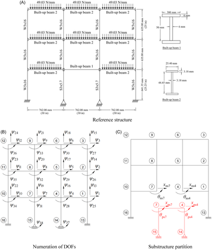
For the partitioned system in RTHS, NS, and PS are interconnected and synchronized via a feedback loop. This allows the force and displacement information to be shared between the two substructures during each time step. In an ideal case, the NS is firstly excited by the earthquake acceleration. Subsequently, the interface nodes displacement responses are obtained by solving Equation (1) and imposed to the PS. Afterward, the generated restoring forces of Equation (2) are measured and returned to the NS. However, due to the typically small vertical displacements of the structure, no vertical displacement is applied in the PS. Instead, only horizontal displacement and rotational displacement are realized. As illustrated in Figure 1C, the DOFs at the common points between the substructures are ${\mathit{\psi }}_{\text{ns}4}={\left[x_{\text{ns}4}{\theta }_{\text{ns}4}\right]}^T$, ${\mathit{\psi }}_{\text{ns}7}={\left[x_{\text{ns}7}{\theta }_{\text{ns}7}\right]}^T$, ${\mathit{\psi }}_{\text{ps}4}={\left[x_{\text{ps}4}{\theta }_{\text{ps}4}\right]}^T$, and ${\mathit{\psi }}_{\text{ps}7}={\left[x_{\text{ps}7}{\theta }_{\text{ps}7}\right]}^T$, where “ps” represents the NS and “ps” represents the PS.

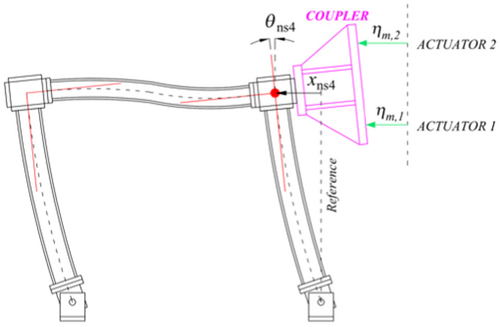
In the benchmark problem, two horizontal actuators are connected to the PS through a coupler. By coordinate transformation, the horizontal and rotational DOFs can be realized, as illustrated in Figure 2. Due to the limitations of the experimental setup, only translational and rotational motions were applied to Node 4.

In real applications, there are various uncertainties such as imprecisions in the geometry of the PS, the material properties, and so forth, as well as measurement noise, and simplified representations of servo-hydraulic actuator dynamics and control–structure interactions [25]. Hence, the maRTHS benchmark problem incorporates uncertainties or model inaccuracies into the control plant. The nominal control plant model follows the form described by Equation (3). In this setting, the poles and zeros of the nominal control plant will undergo random fluctuations, which are derived from the sampling process of the standard normal distribution, thereby resulting in different models. This characteristic gives rise to a series of frequency response functions (FRF), where any member of the FRF can be regarded as a potential instance of the control plant. The nominal values and standard deviation of each parameter are presented in Appendix 1.

3 Principle of RCHP

As discussed in the previous section, a high-precision actuator control strategy can guarantee the success of RTHS. However, there are various sources of uncertainty, including measurement noise, unmodeled inherent dynamics of the hydraulic system, and interactions between the PS and loading system, which can cause the accuracy to decrease and lead to stability issues. To address these challenges, this study proposes RCHP method, as depicted in Figure 4. In this method, the H_∞ loop shaping control enables effective tracking of target displacements, ensures stable dynamic performance of the controlled system, and endows the system with the ability to maintain a relatively constant time delay within a designated frequency band. A classical polynomial extrapolation method is introduced to further mitigate time delay and amplitude discrepancies for the system controlled by the H_∞ controller, which enhances the tracking fidelity.

3.1 H_∞ Loop Shaping Control

In general, the open-loop frequency characteristics are directly related to the steady-state performance, dynamic performance, and noise suppression performance of the closed-loop system. To describe the design goal of the closed-loop system with the open-loop transfer function, one can adjust the shape of the open-loop transfer function in the low-frequency and high-frequency ranges to meet the requirements of system performance and stability margins [26]. The goal of the closed-loop system is to meet the expectations of robust performance and control quality. This is the basic idea of loop shaping.

The H_∞ loop shaping design method fully combines classical loop shaping theory and modern robust control theory. It was proposed by McFarlane and Glover [27] and is a design method based on the coprime factor perturbed plant, according to the small gain theorem and H_∞ theory. It is mainly applied to feedback controller design for systems with unstructured uncertainties.

As shown in Figure 5, the transfer functions from the reference input r to e, y are denoted as S and T, respectively. These are referred to as the system sensitivity function and the complementary sensitivity function. The calculation formulas are as follows:

$$\mathit{S}={(\mathit{I}+\mathit{P}\mathit{K})}^{-1}$$()

$$\mathit{T}=\mathit{P}\mathit{K}{(\mathit{I}+\mathit{P}\mathit{K})}^{-1}=\mathit{I}-\mathit{S}$$()

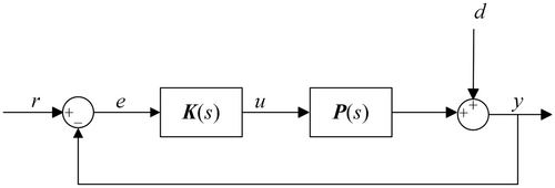
It is apparent that the sensitivity function S serves as a critical metric affecting the response speed of the system. A reduced gain of S is generally associated with enhanced system performance metrics. Conversely, the complementary sensitivity function T acts as a pivotal determinant of the system's robustness. Amplifying the gain of T can significantly attenuate the influence of model uncertainties on the system's performance.

To ensure the RTHS system is endowed with the requirement stated above, a pre-compensator W₁ and a post-compensator W₂ are placed in series with the nominal control plant G to obtain a desired open-loop shape. The shaped plant, G_s, is calculated by

$${\mathit{G}}_{\mathrm{s}}={\mathit{W}}_2\mathit{G}{\mathit{W}}_1\mathbf{.}$$()

When considering the unstructured uncertainties, the RTHS system should be robust and stable. This control problem can be described by coprime factors of the shaped plant, which can be expressed as:

$${\mathit{G}}_{\mathrm{s}}\mathit{=}{(\tilde{\mathit{M}}\mathit{+}{\mathrm{\Delta }}_{\widetilde{\mathit{{\rm M}}}})}^{\mathit{-}1}(\tilde{\mathit{N}}\mathit{+}{\mathit{\Delta }}_{\tilde{\mathit{N}}})$$()

where the transfer matrices $(\tilde{\mathit{M}},\tilde{\mathit{N}})$ are a normalized left coprime factorization of G_s such that ${\mathit{G}}_{\mathrm{s}}={\tilde{\mathit{M}}}^{-1}\tilde{\mathit{N}}$ and $\tilde{\mathit{M}}{\tilde{\mathit{M}}}^{-1}+\tilde{\mathit{N}}{\tilde{\mathit{N}}}^{-1}=\mathit{I}$, and ${\mathrm{\Delta }}_{\tilde{\mathit{M}}}$ and ${\mathrm{\Delta }}_{\tilde{\mathit{N}}}$ are stable but known transfer matrices.

The H_∞ controller needs to ensure that the perturbed system shown in Equation (7) is stable within its perturbation range, and so the controller must satisfy:

$${\mathit{||}\mathit{\left[}\begin{array}{c}\mathit{K}\\ \mathit{I}\end{array}\mathit{\right]}{(\mathit{I}\mathit{-}{\mathit{G}}_{\mathrm{s}}\mathit{K})}^{-1}{\tilde{\mathit{M}}}^{-1}\mathit{||}}_{\infty }\mathit{\le }{\epsilon }^{\mathit{-}1}$$()

The maximum stability margin is calculated by:

$${\epsilon }_{\max }^{-1}\mathit{=}\underset{K\mathit{ }stable}{\text{inf}}{\mathit{||}\mathit{\left[}\begin{array}{c}\mathit{K}\\ \mathit{I}\end{array}\mathit{\right]}{(\mathit{I}\mathit{-}{\mathit{G}}_{\mathrm{s}}\mathit{K})}^{-1}{\tilde{\mathit{M}}}^{-1}\mathit{||}}_{\infty }\mathit{=}{(1\mathit{-}{\mathit{\Vert }{\widetilde{\mathit{{\rm N}}}}_{\mathrm{s}}{\tilde{M}}_{\mathrm{s}}\mathit{\Vert }}_H^2\mathit{)}}^{\mathit{-}1/2}\mathit{=}\sqrt{1\mathit{+}\rho \left(\mathit{X}\mathit{Z}\right)}$$()

where if we let γ = 1/ε, then ${\gamma }_{\min }=\sqrt{1+\rho \left(\mathit{X}\mathit{Z}\right)}$, where ρ is the spectral radius of the matrix, and the matrices X and Z are the positive defined solutions of the following Riccati equation:

$$\begin{array}{l}{({\mathit{A}}_{\mathrm{s}}\mathit{-}{\mathit{B}}_{\mathrm{s}}{\mathit{J}}^{-1}{{\mathit{D}}_{\mathrm{s}}}^T{\mathit{C}}_{\mathrm{s}})}^T\mathit{X}\mathit{+}\mathit{X}({\mathit{A}}_{\mathrm{s}}\mathit{-}{\mathit{B}}_{\mathrm{s}}{\mathit{J}}^{-1}{{\mathit{D}}_{\mathrm{s}}}^T{\mathit{C}}_{\mathrm{s}})\\ \mathit{ }\mathit{-}\mathit{X}{\mathit{B}}_{\mathrm{s}}{\mathit{J}}^{-1}{{\mathit{B}}_{\mathrm{s}}}^T\mathit{X}\mathit{+}{{\mathit{C}}_{\mathrm{s}}}^T{\mathit{R}}^{\mathit{-}1}{\mathit{C}}_{\mathrm{s}}\mathit{=}0\end{array}$$()

$$\begin{array}{l}({\mathit{A}}_{\mathrm{s}}\mathit{-}{\mathit{B}}_{\mathrm{s}}{\mathit{J}}^{\mathit{-}1}{{\mathit{D}}_{\mathrm{s}}}^T{\mathit{C}}_{\mathrm{s}})\mathit{Z}\mathit{+}\mathit{Z}{({\mathit{A}}_{\mathrm{s}}\mathit{-}{\mathit{B}}_{\mathrm{s}}{\mathit{J}}^{\mathit{-}1}{{\mathit{D}}_{\mathrm{s}}}^T{\mathit{C}}_{\mathrm{s}})}^T\\ \mathit{ }\mathit{-}\mathit{Z}{{\mathit{C}}_{\mathrm{s}}}^T{\mathit{R}}^{\mathit{-}1}{\mathit{C}}_{\mathrm{s}}\mathit{Z}\mathit{+}{\mathit{B}}_{\mathrm{s}}{\mathit{J}}^{\mathit{-}1}{{\mathit{B}}_{\mathrm{s}}}^T\mathit{=}0\end{array}$$()

where $\mathit{R}=\mathit{I}+{\mathit{D}}_{\mathrm{s}}{{\mathit{D}}_{\mathrm{s}}}^T$, $\mathit{J}=\mathit{I}+{{\mathit{D}}_{\mathrm{s}}}^T{\mathit{D}}_{\mathrm{s}}$. In Equations (10) and (11), A_s, B_s, C_s, and D_s are stabilizable and detectable state space realizations of the shaped plant.

Once reaching a reasonable γ_min, the H_∞ controller can be calculated by:

$$\mathit{K}\mathit{=}\mathit{\left[}\begin{array}{ll}{\mathit{A}}_{\mathrm{K}}& {\mathit{B}}_{\mathrm{K}}\\ {\mathit{C}}_{\mathrm{K}}& {\mathit{D}}_{\mathrm{K}}\end{array}\mathit{\right]}$$()

where

$${\mathit{A}}_{\mathrm{K}}\mathit{=}{\mathit{A}}_{\mathrm{s}}\mathit{+}{\mathit{B}}_{\mathrm{s}}\mathit{F}\mathit{+}{\gamma }^2{\mathit{\left(}{\mathit{L}}^T\mathit{\right)}}^{\mathit{-}1}\mathit{Z}{{\mathit{C}}_{\mathrm{s}}}^T\mathit{(}{\mathit{C}}_{\mathrm{s}}\mathit{+}{\mathit{D}}_{\mathrm{s}}\mathit{F}\mathit{)}$$()

$${\mathit{B}}_{\mathrm{K}}\mathit{=}{\gamma }^2{\mathit{\left(}{\mathit{L}}^T\mathit{\right)}}^{\mathit{-}1}\mathit{Z}{{\mathit{C}}_s}^T$$()

$${\mathit{C}}_{\mathrm{K}}\mathit{=}{{\mathit{B}}_{\mathrm{s}}}^T\mathit{X}$$()

$${\mathit{D}}_{\mathrm{K}}\mathit{=}\mathit{-}{{\mathit{D}}_{\mathrm{s}}}^{\mathit{T}}$$()

and $\mathit{F}\mathit{=}\mathit{-}{\mathit{J}}^{-1}\mathit{(}{{\mathit{D}}_{\mathrm{s}}}^T{\mathit{C}}_{\mathrm{s}}\mathit{+}{{\mathit{B}}_{\mathrm{s}}}^T\mathit{X}\mathit{)}\mathit{,}\mathit{L}\mathit{=}(1\mathit{-}{\gamma }^2\mathit{)}\mathit{I}\mathit{+}\mathit{X}\mathit{Z}$.

4 Controller Design and Validation

4.1 Controller Design

4.1.1 H_∞ Loop Shaping Controller

When designing the H_∞ loop shaping controller, the following considerations should be made for the desired open-loop transfer function. A high gain is needed in the low-frequency range to obtain better tracking performance. The slope of the descent in the mid-frequency range should not be too large; close to −20 dB/dec is ideal. In the high-frequency range, it should have a faster attenuation to reduce the influence of noise. The selection of the compensator often requires a certain amount of experience, and the robust stability and dynamic performance need to be comprehensively considered. When the stability margin value lies between 1 and 3, the trade-off design between the system's dynamic performance and robustness is better. If γ_min > 10, this indicates that the selected pre- and/or postcompensators are inappropriate and need to be reselected. For control problems in multi-input multi-output systems, it is studied that choosing compensators as diagonal matrices helps reduce the complexity and coupling effects inherent in multivariable systems [29]. This approach facilitates approximate decoupling between distinct control objectives, thereby enabling independent tuning and control for each individual channel. In this study, the compensators are selected as the diagonal matrix, and after several trials, the pre- and postcompensators are chosen as:

$${\mathit{W}}_1\mathit{=}\mathit{\left[}\begin{array}{cc}\frac{22.5s\mathit{+}520}{s\mathit{+}0.01}& 0\\ 0& \frac{2.8s\mathit{+}400}{s\mathit{+}0.01}\end{array}\mathit{\right]}$$()

$${\mathit{W}}_2\mathit{=}\mathit{\left[}\begin{array}{cc}\frac{0.057s+1}{0.04s+1}& 0\\ 0& \frac{0.0425s+1}{0.028s+1}\end{array}\mathit{\right]}\mathit{.}$$()

Finally, the H_∞ controller is obtained and the γ value is 2.2489, indicating that there is a good trade-off between the robust stability and dynamic performance of the controlled system.

Figure 6 presents the transfer functions S, T, and GK of the controlled system. It can be seen that GK has a relatively high gain in the low-frequency range, indicating good tracking performance. When the singular value curve crosses 0 dB, the slope is −20 dB/dec, which ensures the steady-state performance of the system. In the high-frequency range, the singular value curve decays rapidly at a slope of at least −40 dB/dec, which can effectively suppress the influence of noise. The complementary sensitivity function T has singular values close to 0 in the low-frequency range, indicating strong tracking performance. Moreover, T decays rapidly in the high-frequency range, suggesting that the influence of modeling errors is reduced. The system sensitivity function S has a relatively low gain in the low-frequency range, demonstrating effective suppressing of disturbances in the low-frequency range.

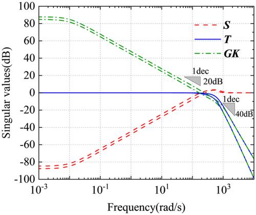
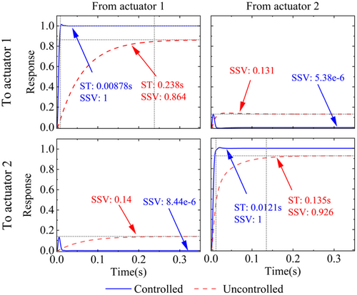
Figure 7 displays the step responses of the controlled system with and without the H_∞ controller. The settling times (ST) of the proposed method are 0.00878 s and 0.0121 s; in contrast, the settling times of the uncontrolled system are 0.238 s and 0.135 s, significantly slower. The steady-state error of the controlled system is almost negligible, exhibiting excellent tracking performance; in comparison, the steady-state values (SSV) of the uncontrolled system are 0.864 and 0.926, with relatively large steady-state errors and poor tracking performance. The off-diagonal subplots reflect the coupling between actuators. It can be seen from this figure that the coupling only appears in the short transition stage, and then weakens rapidly, with the final steady-state value being close to zero. In contrast, the coupling effect of the uncontrolled system is significant and stabilizes at a relatively large value, indicating that its coupling is relatively strong. That is to say, the proposed method can achieve approximate decoupling among actuators, and it is rational of applying the PE module to each actuator individually in the following design process.

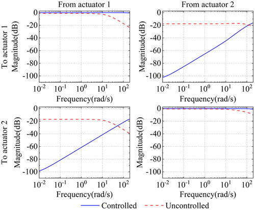
The amplitude-frequency plots of the controlled and uncontrolled systems are given in Figure 8. The figures reveal that the amplitude of the uncontrolled system is relatively small in the low-frequency range, and decreases rapidly in the mid-frequency range, indicating poor tracking performance. The amplitude of the controlled system is essentially maintained near 0 dB in the middle- and low-frequency ranges, which effectively ensures the tracking performance of the system. The off-diagonal subplots show the amplitude-frequency characteristics of the coupling effect. Obviously, the coupling amplitude of the controlled system in the middle- and low-frequency ranges is significantly smaller than that of the uncontrolled system, and is only slightly higher than that of the uncontrolled system within a relatively small frequency band, indicating that the proposed method has a certain decoupling effect.

4.2 Polynomial Extrapolation

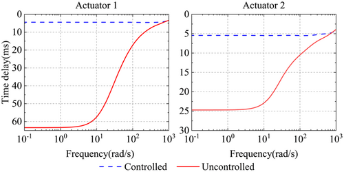
Figure 9 illustrates the system delays of the H_∞ control system and the uncontrolled system. As observed in the figure, within the 100 rad/s frequency range, the delays for the two actuators in the uncontrolled system fluctuate significantly, ranging from 17.6 ms to 63.4 ms and from 10.5 ms to 24.7 ms, indicating substantial variability and longer delays. In contrast, the delays in the controlled system are nearly linear, remaining consistently low at approximately 4.4 ms and 5.45 ms for the two different actuators, respectively. These results demonstrate that the H_∞ controller effectively mitigates the high amplitude variations in delay experienced by the uncontrolled system, and maintains the delays in the controlled system at a low level within the frequency range under consideration. Hence, the PE method can be introduced to further reduce the system time delay.

Thus, the relatively constant delays of the two actuators within the 100 rad/s range (specifically 4.4 ms and 5.45 ms) are substituted into the polynomial extrapolation expression in Equation (17). Consequently, the computed η values for the polynomial extrapolation are 4.506 and 5.581, respectively.

At this point, the proposed controller design is complete.

4.3 Tracking Performance Validation

To verify the tracking performance of RCHP method, a virtual simulation model based on the designed controller was established in the MATLAB/Simulink environment. A specified displacement was used as the input signal. When obtaining this displacement, the Kobe earthquake record (with a peak ground acceleration [PGA] scaled to 0.4 g) was employed as the excitation source to drive the benchmark reference structure for a comprehensive analysis, resulting in displacement and rotation at the boundary of the PSs. Subsequently, after coordinate transformation, the desired displacement was obtained.

To facilitate a comparative analysis of the proposed method's performance, three control schemes are considered: H_∞ control, RCHP, and a baseline control strategy known as LQG control, for specified displacement tracking.

Figure 10 illustrates the tracking time histories for the three control methods. It is evident that the tracking displacements from all three approaches are similar. Further analysis reveals that the tracking curve under just H_∞ control exhibits significant time delays. However, with the introduction of the second stage of control (i.e., polynomial extrapolation), the influence of these delays is effectively mitigated, resulting in a notable improvement in the alignment of the tracking curve with the reference value, thereby validating the efficacy of the PE method. In the LQG control scenario, the discrepancies in the tracking curves are particularly pronounced at the peak values. Conversely, with the RCHP control approach, the errors at the peak are significantly reduced, enhancing the degree of conformity. The tracking curves of the two actuators were compared, revealing that under LQG control, Actuator 2 exhibited significantly poorer tracking performance compared to Actuator 1. However, when the RCHP control was applied, both Actuator 2 and Actuator 1 achieved excellent tracking performance.

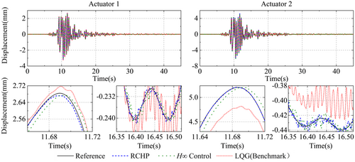
In addition, we calculate three tracking performance evaluation metrics for the two actuators: time delay (J₁), normalized tracking error (J₂), and maximum peak tracking error (J₃). The calculated results are presented in Table 1.

Table 1. Performance evaluation.

	J1/ms		J2/%		J3/%
Actuator	1	2	1	2	1	2
LQG	1.9531	2.9297	4.0809	8.7873	3.7761	8.9177
H∞ control	3.9063	5.8594	5.7006	7.3539	6.5798	8.0318
RCHP	−0.9766	0.0000	2.9809	1.5226	2.0221	0.9317

• Abbreviations: LQG, linear quadratic Gaussian; RCHP, robust compensation strategy combining H_∞ control theory and polynomial extrapolation.

As presented in Table 1, the data therein reveal that the H_∞ control method manifests a discernible degree of time delay. The tracking errors of J₂ and J₃ suggest that the H_∞ control method has relatively poor tracking performance. Conversely, the LQG control method showcases some improvements regarding time delay and tracking error. For instance, the time delays are lower compared to those of the H_∞ control method. Although there is an improvement, the relatively high error values still imply that there is room for further optimization in its tracking performance. Among the three control methods, the RCHP control approach demonstrates outstanding performance. The time delays are reduced to near-zero levels, indicating an almost perfect compensation effect. The negative time delay value for Actuator 1 might be attributed to the effect of measurement noise. Compared to H_∞ control, the J₂ values for Actuator 1 and Actuator 2 are reduced by 47.7% and 79.3%, respectively, while the J₃ values reduced by 69.6% and 88.4%, respectively. This verifies the efficacy of the PE in reducing time delay. When implementing the RCHP method, the J₂ values for Actuator 1 and Actuator 2 are reduced to 73.0% and 17.3% of those obtained with the LQG benchmark control strategy, respectively. Regarding J₃, the maximum absolute deviations for the two actuators exhibited a significant reduction, reaching 53.5% and 10.4% of the LQG method's corresponding values. The aforementioned data demonstrate that the RCHP has achieved a marked improvement in time synchronization and tracking accuracy, providing a reliable solution for high-precision control in maRTHS.

5 Virtual Real-Time Hybrid Simulations

To verify the feasibility and effectiveness of the RCHP, a series of virtual RTHSs (vRTHS) were conducted based on the virtual maRTHS benchmark model proposed by Condori et al. [24] The RCHP presented in Section 3.1 and the benchmark LQG controller configured for the model were used for these tests.

5.1 Tracking Performance

The tracking performance of the RCHP was validated using the El Centro earthquake excitation with the PGA scaled to 0.4 g as the input. Figure 11 presents the time-history curves of the measured and desired displacements of two actuators during a single vRTHS test on the nominal control plant. It can be seen in Figure 11A, the LQG method exhibits significant deviations at peak values and a noticeable time delay near zero displacement. In contrast, Figure 11B illustrates the measured and target displacements for RCHP, demonstrating significantly smaller errors at peak values, particularly for Actuator 2. Moreover, the proposed method exhibits less time delay near zero displacement and closely aligns with the target displacement. These results indicate that RCHP effectively tracks the target displacement and successfully addresses the time delay issues commonly encountered in multi-boundary-point real-time hybrid simulations.

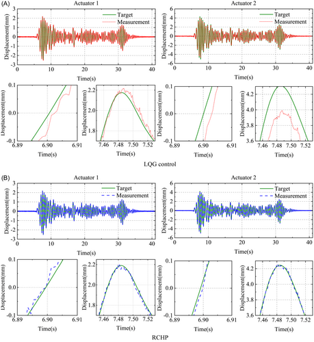
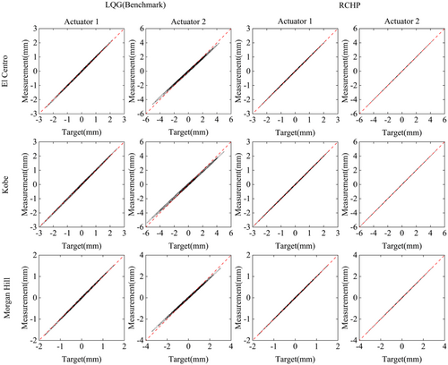
Figure 12 presents the synchronization subspace plots of the actuators under the El Centro, Kobe, and Morgan Hill earthquake excitations for the LQG control method and RCHP method. The displacement relationship curves of the LQG control method are relatively scattered for all three seismic inputs, with pronounced hysteresis loops, indicating poor tracking performance and a low level of agreement between the target and measured displacements. Notably, in the LQG-controlled Actuator 2, there is a distinct angular deviation from the 45-degree reference line. This deviation quantifies a significant tracking amplitude error, revealing the inefficiency of LQG in precisely tracking the desired displacement for Actuator 2. In contrast, the displacement relationship curves of RCHP method are much narrower. They closely approximate the 45-degree diagonal, which is the ideal alignment for perfect tracking. This indicates that the RCHP method can accurately track the target displacement, minimizing the error between the measured and desired values. Thus, it showcases excellent tracking performance in vRTHS, outperforming the LQG control method.

5.2 Assessment Criteria

The benchmark problem defined 10 performance metrics to quantitatively assess the accuracy and effectiveness of different control methods. The evaluation metrics are categorized into two groups: (1) J₁–J₆ as tracking performance metrics and (2) J₇–J₁₀ as global performance metrics. Among these, J₁–J₃ assess the error between the measured displacement and the target displacement, while J₄–J₆ evaluate the error between the estimated displacement and the target displacement. Metrics J₇–J₁₀ analyze the measured and reference displacements of the second and third floors of the frame. J₁ and J₄ are expressed in milliseconds (ms), while the remaining metrics are expressed as percentages (%). The formulas for all metrics are provided in Appendix 1.

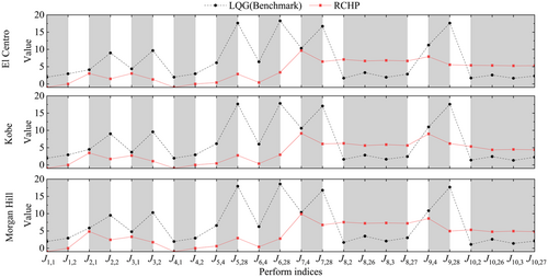
The El Centro, Kobe, and Morgan Hill ground motions, each with a PGA of 0.4 g, were selected as inputs to perform vRTHS analysis on the nominal control plant, employing both RCHP method and the LQG method. A total of 24 error metric values were calculated, as presented in Figure 13. In the abscissa, the first subscript denotes the metric index (J₁–J₁₀), while the second subscript specifies actuator numbers for J₁–J₄ and structural DOFs for J₅–J₁₀. As shown in the figure, RCHP achieves near-zero calculated time delays for both actuators, outperforming LQG method. Across all actuators, RCHP reduces delays by almost 100% compared to LQG. Regarding the tracking performance metrics J₂–J₆, RCHP demonstrates superior precision, with errors reduced by 17.4%–100%. For instance, taking the error metric J₆ at the 28th DOF under the El Centro earthquake excitation as an example, the calculated value of the RCHP method is merely about 13% of that of the LQG method. For the error metrics of the second and third floors (J₈ and J₁₀), the proposed method shows slightly higher values than the LQG method. This can be attributed to the relatively complex coordinate transformations and signal differentiations in the benchmark model. These operations might amplify certain signals, thereby increasing the overall indicators. Overall, the RCHP method generally produces smaller evaluation metrics compared to the LQG method, demonstrating its superiority in maRTHS.

To systematically evaluate the robustness of the RCHP method under modeling uncertainties and varying input excitations, 600 vRTHS tests (200 trials per seismic excitation) were conducted using El Centro, Kobe, and Morgan Hill ground motions (PGA of 0.4 g). Figure 14 illustrates the distribution histograms and cumulative distribution function (CDF) plots of tracking evaluation metrics. The diverse ground motions cause discrepancies in the centers of the metric distributions. This is expected since each ground motion imparts distinct dynamic forces on the system, leading to different responses. Multiple peaks are observable in metrics like J_2,1, J_2,2, J_5,4, and J_6,28. Nonetheless, upon a detailed and in-depth analysis, it is evident that the metrics remain concentrated even under different ground motions, with distinct peaks, small data fluctuations, and rapid increases in CDF. Specifically, the values of J₂ and J₃ for Actuator 1 are both less than 6.5%, while those for Actuator 2 are below 2.5%. Similarly, the values of J₅ and J₆ for DOF 4 are both less than 0.65%, while those for DOF 28 are below 3.1%. These results indicate that the RCHP method is minimally affected by variations in seismic excitation characteristics and modeling uncertainties, demonstrating its reliability and resilience as a control strategy for maRTHS.

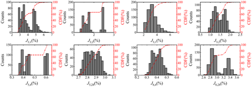
Table 2 presents the nominal values, mean values, and standard deviations (SD) of evaluation metrics J₇–J₁₀ for the RCHP method across 200 vRTHS tests conducted for each seismic excitation, amounting to a total of 600 tests. It is evident that the mean values of J₇ and J₉ for RCHP method are lower than those of the LQG method. For example, in the case of the El Centro seismic excitation, the mean values of J₇ for the RCHP method are 9.65% and 6.48%, while for the LQG method, they are 10.44% and 16.81%, suggesting a better performance in certain aspects. However, RCHP shows slightly higher mean values for relative displacement errors in J₈ and J₁₀, which is similar with that in the nominal case. It should be noted that the differences between the mean values and nominal values are small for both methods. However, further analysis reveals that the maximum standard deviation of RCHP method is only 0.074, with a minimum of 0.005, whereas the LQG control method has a maximum standard deviation of 1.344 and a minimum of 0.014. Taking the Kobe excitation as an example, the standard deviation of J₈ is only 1.7% of that for LQG (0.750), indicating that RCHP reduces sensitivity to model uncertainties by two orders of magnitude. The results imply that the RCHP method reduces sensitivity to uncertainties in the system. This enhanced stability under different seismic inputs is a strong indicator of the RCHP method's higher robustness compared to the LQG control method. In practical terms, it suggests that the RCHP method is more reliable, making it a more favorable option for applications in maRTHS scenarios.

Table 2. Nominal, average, and standard deviation of global performance.

Ground motions	Method	Classification	J7,4(%)	J7,28(%)	J8,2(%)	J8,26(%)	J8,3(%)	J8,27(%)
El Centro	LQG	Nominal	10.33	16.69	1.67	3.26	1.92	2.83
		Average	10.44	16.81	1.67	3.26	1.92	2.83
		SD	1.096	1.344	0.024	0.032	0.031	0.032
	RCHP	Nominal	9.65	6.48	7.09	6.66	6.82	6.66
		Average	9.65	6.48	7.09	6.66	6.82	6.66
		SD	0.005	0.013	0.017	0.019	0.018	0.019
Kobe	LQG	Nominal	10.62	17.05	1.63	2.84	1.65	2.43
		Average	10.78	17.24	1.63	2.84	1.65	2.43
		SD	0.617	0.750	0.014	0.023	0.022	0.023
	RCHP	Nominal	9.13	6.09	6.24	5.62	5.89	5.64
		Average	9.13	6.09	6.24	5.62	5.89	5.64
		SD	0.005	0.013	0.014	0.017	0.015	0.017
Morgan	LQG	Nominal	10.36	16.79	1.69	3.50	2.08	3.04
		Average	10.65	17.14	1.69	3.50	2.08	3.04
		SD	0.990	1.204	0.024	0.032	0.031	0.032
	RCHP	Nominal	9.91	6.75	7.55	7.22	7.33	7.21
		Average	9.91	6.75	7.55	7.22	7.33	7.21
		SD	0.005	0.013	0.018	0.022	0.02	0.021

Ground motions	Method	Classification	J9,4(%)	J9,28(%)	J10,2(%)	J10,26(%)	J10,3(%)	J10,27(%)
El Centro	LQG	Nominal	11.25	17.61	1.70	2.56	1.64	2.28
		Average	11.28	17.65	1.70	2.56	1.64	2.28
		SD	0.520	0.700	0.020	0.019	0.021	0.022
	RCHP	Nominal	7.91	5.56	5.39	5.35	5.26	5.29
		Average	7.89	5.63	5.39	5.35	5.26	5.29
		SD	0.038	0.044	0.015	0.015	0.015	0.014
Kobe	LQG	Nominal	10.99	17.57	1.40	2.43	1.33	2.23
		Average	11.14	17.78	1.40	2.43	1.33	2.23
		SD	0.323	0.432	0.015	0.016	0.015	0.016
	RCHP	Nominal	8.99	6.19	5.34	4.37	4.48	4.39
		Average	8.98	6.11	5.34	4.37	4.48	4.39
		SD	0.032	0.047	0.01	0.013	0.01	0.013
Morgan	LQG	Nominal	10.86	17.69	1.10	2.60	1.39	2.08
		Average	10.81	17.61	1.10	2.60	1.40	2.08
		SD	0.646	0.883	0.020	0.019	0.020	0.021
	RCHP	Nominal	8.61	4.96	5.32	4.78	4.95	4.79
		Average	8.70	5.00	5.31	4.78	4.95	4.80
		SD	0.042	0.074	0.01	0.015	0.013	0.015

• Abbreviations: LQG, linear quadratic Gaussian; RCHP, robust compensation strategy combining H_∞ control theory and polynomial extrapolation; SD, standard deviation.

6 Conclusions

While the virtual RTHSs validate RCHP's theoretical advantages, physical implementation remains untested. Future studies should incorporate experimental verification under diverse loading conditions and nonlinear structural behaviors. Additionally, extending the framework to adaptive compensation designs, incorporating machine learning, or nonlinear extrapolation techniques could enhance its versatility for broader engineering applications.

Conflicts of Interest

The authors declare no conflicts of interest.