Volume 4, Issue 1 pp. 76-96

RESEARCH ARTICLE

Full Access

Probabilistic Seismic Hazard Assessment of Palghar District, Maharashtra, India by Considering Spatially Nonuniform Seismicity

Suman Sinha,

Corresponding Author

Suman Sinha

orcid.org/0000-0002-4071-7634

Engineering Seismology Division, Central Water and Power Research Station, Pune, India

Correspondence: Suman Sinha ([email protected]; [email protected])

Search for more papers by this author

S. Selvan,

S. Selvan

Engineering Seismology Division, Central Water and Power Research Station, Pune, India

Search for more papers by this author

Sachin Khupat,

Sachin Khupat

Engineering Seismology Division, Central Water and Power Research Station, Pune, India

Search for more papers by this author

Rizwan Ali,

Rizwan Ali

Engineering Seismology Division, Central Water and Power Research Station, Pune, India

Search for more papers by this author

Suman Sinha,

Corresponding Author

Suman Sinha

orcid.org/0000-0002-4071-7634

Engineering Seismology Division, Central Water and Power Research Station, Pune, India

Correspondence: Suman Sinha ([email protected]; [email protected])

Search for more papers by this author

S. Selvan,

S. Selvan

Engineering Seismology Division, Central Water and Power Research Station, Pune, India

Search for more papers by this author

Sachin Khupat,

Sachin Khupat

Engineering Seismology Division, Central Water and Power Research Station, Pune, India

Search for more papers by this author

Rizwan Ali,

Rizwan Ali

Engineering Seismology Division, Central Water and Power Research Station, Pune, India

Search for more papers by this author

First published: 31 March 2025

https://doi.org/10.1002/eer2.70000

Share a link

Email
Wechat
Bluesky

ABSTRACT

The Palghar district of Maharashtra has recently received attention because of frequent occurrences of earthquakes in its vicinity in the last few years since November 2018. The district falls under seismic zone III, as per the seismic zonation map of India. As the recent earthquake activities have been preceded by many major seismic events in the region, it necessitates to re-evaluate the level of seismic hazard of the area in a reliable and realistic way. With this aim in mind, the probabilistic seismic hazard map of Palghar district with regard to Peak Ground Acceleration (PGA) and $5 %$ damped pseudo-spectral acceleration (PSA) at $0.2$ and $1.0$ s for $10 %$ and $2 %$ probability of exceedance (PoE) in $50$ years at engineering bedrock level is presented. The estimation of hazard is performed in a finer grid resolution of 0.02° $\times$ 0.02° and takes into consideration the nonuniform distribution of earthquake probability within a seismic source zone (SSZ) and data-driven selection of suitable ground motion prediction equations (GMPEs) with appropriate weight factors. The spatial variation of the hazard level as reflected in the hazard maps, demonstrates notable improvements over the earlier studies. The PGA at the atomic power plant in the district is found to be 0.15 g for DBE condition. The results can be used for designing earthquake-resistant structures in addition to assessing seismic safety of the existing structures.

1 Introduction

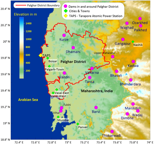
Palghar district lies in the Konkan division of Maharashtra State and Palghar town is the administrative capital of the Palghar district. Palghar is considered to be a district of economical significance in India and is an industrial hub, too. It is home to India's first atomic power plant, Tarapur Atomic Power Station (TAPS). The busy Mumbai–Ahmedabad rail corridor passes through this district. Moreover, a number of dams are housed in and around the Palghar district. In the last 4 years, Palghar region witnessed an unusual frequency of earthquakes. Srinagesh et al. [1] stated that around 4854 events in the magnitude range 0.1 $M_{L}$ to 4.1 $M_{L}$ of focal depths ranging from 4 to 16 km during the period January 30, 2019 to August 31, 2019. Within the Palghar district boundary, 34 events having magnitude M_L 3.0 to M_L 4.1 have been reported by the National Centre for Seismology, Government of India, during the period November 2018 to October 2019. The largest ( $M_{L}$ 4.1) among them took place on March 1, 2019 and eight earthquakes in the magnitude range $M_{L}$ 3.1–3.7 were recorded on February 1, 2019 at a span of 8 h. Although Palghar district falls under Peninsular shield which lies in the stable continental region (SCR) of the Indian Subcontinent, the same has witnessed few major earthquakes in the past. These include Bhuj earthquake ( $M_{W}$ 7.6, 2001), Jabalpur earthquake ( $M_{W}$ 5.8, 1997), Latur earthquake ( $M_{W}$ 6.1, 1993), and Koyna earthquake ( $M_{W}$ 6.4, 1967) which caused enormous loss of lives and extensive damage to properties. Therefore, re-evaluation of seismic safety to assess the vulnerability of important structures against earthquakes is very much necessary for this region. Map showing the boundary of Palghar district along with the locations of important structures in its vicinity are shown in Figure 1.

Details are in the caption following the image — **Figure 1**
Open in figure viewer PowerPoint

The geographical boundary (approximate) of Palghar district and locations of the dams and Tarapore Atomic Power Station (TAPS).

Seismic safety is generally evaluated in terms of seismic hazards which are quantified by the determination of different ground motion parameters. The ground shaking associated with earthquakes plays the most vital role [2]. It inhabits in area prone to earthquakes with favorable seismo-tectonics and local geological site characteristics, causing significant damage to properties and lives. It necessitates estimating the terrain's seismic hazard realistically to derive the essential design criteria for building earthquake-resistant structures. The sudden recent seismic activities, discussed earlier, together with the past damaging earthquakes motivate us to quantify seismic hazard in a realistic approach.

The Indian Standard for criteria for earthquake resistant design of structures [3], that is, the Indian Seismic Regulations, primarily deals with earthquake-resistant design of various structures. This Indian Standard [3] divides entire India into four seismic zones, having different zone factors for the purpose of design seismic force. The zone factor is double the ZPA of the design factor. The present study area falls in seismic zone III, having zone factor 0.16. This Seismic Regulations also give a standard design acceleration coefficient for different soil types (Rock or hard soils, Medium or Stiff soils, and soft soils), normalized with respect to PGA, corresponding to the natural period of the structure. But the main limitation of the Indian seismic zonation code, as presented in BIS [3] is that it lacks probabilistic features [4] and hence it isn't grounded in a thorough seismic hazard analysis. But given its solid scientific foundation [2], the probabilistic approach to seismic hazard calculation is thought to be more appropriate. Taking into account the randomness of earthquake occurrences in space, time, and magnitude, the ground motion, estimated using the PSHA method with a pre-defined confidence level, will not exceed at any time period due to any anticipated earthquake over a fixed period of time. The mathematical expression of PSHA was formed by Cornell [5] and McGuire [6].

Although some authors (Khattri et al. [4]; Bhatia et al. [7]; Iyengar et al. [8]; Nath and Thingbaijam [9]; Sitharam and Kolathayar [10]; Kolathayar and Sitharam [11]; Ghosh et al. [12]) performed the PSHA study of entire India on a macro-scale level, region-specific PSHA study for Peninsular India (PI) started after 2007 (Anbazhagan et al. [13]). These studies were carried out by Jaiswal and Sinha [14], Kanagarathinam et al. [15], Anbazhagan et al. [16], Vipin et al. [17], Rohan and Basu [18], Menon et al. [19], Anbazhagan et al. [20], Sitharam et al. [21], Ashish et al. [22], Scaria et al. [23]. In all of these studies, except Scaria et al. [23], the GMPEs were used without performing a suitability analysis and therefore ranking and weights of GMPEs, which are very important for seismic hazard studies, were absent in those studies. In most of these studies, the GMPE, developed by Raghukanth and Iyenger [24], was considered superior and more weight was given. However, the present study reveals that the GMPE due to Raghukanth and Iyenger [24] yields a higher LLH scores compared to the other selected GMPEs. Same conclusion was drawn by Scaria et al. [23] about the use of GMPE developed by Raghukanth and Iyenger [24]. Although Scaria et al. [23] had discussed the ranking of GMPEs, the authors finally chose an old GMPE of Abrahamson and Silva [25] with some modification of the amplitude term. Some studies used GMPEs which date back to 1997. Most of the studies did not consider the minimum criteria proposed by Cotton et al. [26] and Bommer et al. [27] for primary selection of GMPEs. In our study, following the minimum criteria proposed by Cotton et al. [26] and Bommer et al. [27], 16 GMPEs have been primarily selected for performing the efficacy test and ranking of the GMPEs. The values of different ground motion parameters depend a lot on the choice of the GMPEs. Therefore, selection of appropriate GMPEs for a specific area is very crucial in any study on seismic hazard. The present work has addressed this issue by carrying out a detailed quantitative assessment for selection of suitable GMPEs.

As the seismicity is, in general, diffused in nature in Peninsular shield, the rates of occurrence of expected earthquakes in different magnitude ranges are distributed non-uniformly over equally spaced grids of interval as per the smoothed epicentral density of observed past earthquakes. The approach is known as smooth-gridded seismicity model after Frankel [28]. On the contrary, the conventional uniform seismicity model assumes same earthquake occurrence rates for all the grid points inside a seismic source zone (SSZ), which either underestimates or overestimates the earthquake occurrence rates, depending upon the locations of past earthquakes. In this study, the grid interval is taken as 0.02° $\times$ 0.02°. The seismic hazard computations at grid intervals of higher resolution have been performed after assessing the suitability of various GMPEs against observed accelerograms using log-likelihood (LLH) score introduced by Scherbaum et al. [29].

At engineering bedrock (which conforms to $V_{s 30}$ value∼760 m/s), the spatial distribution of PGA and $5 %$ damped PSA at specific time periods for $10 %$ and $2 %$ probability of exceedance (PoE) in $50$ years corresponding to return periods $475$ years, known as design basis earthquake (DBE) and $2475$ years, known as maximum credible earthquake (MCE), respectively have been obtained [30, 31]. The periods 0.2 and 1.0 s are commonly used as corner periods to construct a response spectrum for structural design [9, 32]. Although the PSA at all the periods have been computed, the PSA at 0.2 and 1.0 s along with PGA are used to construct the response spectra in the present work [32]. The resulting hazard maps show the spatial variations in seismic hazard of Palghar district. It is expected that the findings will assist governments in making decisions about disaster mitigation and be beneficial to structural engineers in designing earthquake-resistant structures.

2 Seismo-Tectonic Setup of the Area of Study

Seismic hazard assessment of Palghar district requires evaluating regional seismicity within a buffer of 300 km from its geographical boundary. The study area is defined as being between 16.5° N–23.5° N in latitude and 69.5° E–76.5° E in longitude. Figure 2 displays the main seismo-tectonic features in the study area based on the Seismotectonic Atlas of India and Its Environs (SEISAT), which was released by Geological Survey India (GSI) [33]. The structural trends in the region is comprised of northern portion of NW trending Western Ghats, Deccan Plateau and Son Narmada, and Tapti Rift Zones. The NW trending Western Ghats is one of the major uplifted plateaus in the Indian Shield. The Ghats span a wide variety of geological formations with varying structural and physical properties. One of the main tectonic features in the Ghats is the West-Coast Fault, which is naturally the divide between the Indian plate and Gondwanaland. The East Marginal Fault of the Cambay Graben may be continuous with this feature. Relative to the West Coast Fault, the Chiplun Fault is thought to represent its secondary manifestation. One additional significant tectonic feature in this zone is the monoclonal Panvel Flexure, which has a western limb that dips toward the west. This flexure trends parallel to the West Coast Fault [33] in a NNW direction along its axial track. Major faults and lineaments in the Deccan Plateau area trend NW-SE, which is in line with the tectonic grains of the nearby Precambrian basement rocks. It is discovered that some of the faults and lineaments that cross the trap rocks continue into the older rocks that surround them. The Neo Tectonic Fault (Ghod), the Upper Godavari Faults (UGF), and a few other faults with basement and cover are the main geofractures in this zone. The presence of transverse faults are the indication of the abrupt changes in Deccan Trap thickness and base level depths. It has been identified that the Son Narmada South Fault (NSF), which is trending ENE-WSW, is episodically active. The Narmada North Fault (NNF) and NSF are the constituents of the boundary fault systems that control the Narmada Rift Basin in the area. These faults extend up to the mantle and have been reactivated many times in the past. The Barwani-Sukta Fault and the Tapti North Fault (TNF) have a parallel curved E-W to ENE-WSW appearance. TNF continues along the southern portion of the Satpura axial zone, branching out to the east into the Gavilgarh Fault, another ENE-WSW facing fault that stretches northeast of Akot and edges out the northern tectonized margin of the Purna alluvium. Some parts of the Narmada South and the TNF exhibit neotectonism. The Son-Narmada Fault and TNF have ENE-WSW trend, and extends beyond the Cambay Graben to enter the Saurashtra Peninsula towards west. TNF characterizes the southern border of the Satpura range and northern border of Tapti alluvium. The Kaddam Fault, gets terminated by the Purna Fault, the southernmost fault of Son-Narmada-Tapti (SONATA) lineament Zone [33]. To correlate historical seismicity with the existing tectonic features, the epicenters of the main shocks are overlaid on the tectonic features in Figure 2.

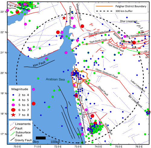
A number of moderate to large earthquakes have been recorded in the study region in the past. Table 1 shows the list of few significant earthquakes having magnitudes above 5.5 Mw. Among them, the 5.7 Mw event of December 25, 1856 occurred at a distance of around 20 km from TAPS. The 7.0 Mw Bhavnagar earthquake of February 02, 1705 and 6.4 Mw Koyna earthquake of December 10, 1967 occurred at a large distance of more than 200 km from the Palghar district. The seismic activities in the Palghar district are attributed to the presence of Panvel Flexure, the northern limp of the West-Coast Fault, and the western limp of the Ghod Fault. Sporadic seismic activities in the past have also been reported around the location of the current activities. Reservoir-induced seismicity was reported at the Dhamini reservoir, which began in 1984 and continued up to 1986. The seismic activities were paused and got reactivated in 1994, continuing till 1995. During this period, 69 events with magnitudes around 3.0 have been recorded [1]. Even though there is no record of large earthquake in Palghar district in the recent past, the largest historic event recorded in the district is 5.7 Mw event of December 25, 1856.

Table 1. Few significant historic earthquakes in the study region.

Date	Region	Lat ( $° N$ )	Lon ( $° E$ )	Magnitude ( $M_{W}$ )
May 26, 1618	Mumbai, Maharashtra	18.90	72.90	6.5
February 04, 1705	Bhavnagar, Gujarat	22.70	72.30	7.0
August 18, 1764	Koyna, Maharashtra	17.90	73.70	6.0
December 25, 1856	Palghar region, Maharashtra	20.00	72.70	5.7
April 29, 1864	Kathiawar, Gujarat	22.30	72.80	5.7
April 21, 1919	Hebatpur, Gujarat	22.00	72.00	6.2
April 08, 1951	Konkan area, Maharashtra	18.50	70.80	6.0
December 13, 1957	Koyna, Maharashtra	17.30	73.70	6.1
December 10, 1967	Koyna, Maharashtra	17.54	73.84	6.4

3 Methodology

3.1 Earthquake Catalogue

The preparation of an earthquake catalogue is the initial step in the assessment of seismic hazards. The term “earthquake catalogue” refers to an earthquake database that includes information about each individual earthquake event, with its time of occurrence (year, month, day, hour, and minute), location (longitude, latitude, and depth), and magnitude ( $M_{L}$ —local magnitude, $M_{S}$ —surface wave magnitude, $m_{b}$ —body wave magnitude and $M_{W}$ —moment magnitude). For the present analysis, the earthquake catalogue for the instrumental period has been prepared using the data available from the National Earthquake Information Centre (NEIC), the United States Geological Survey (USGS), the reviewed International Seismological Centre (ISC) bulletin, UK and National Center for Seismology (NSC), India. For pre-instrumental and early instrumental period, the data has been obtained from various published sources [34-37]. There are $714$ events in the catalogue compiled for this study, which begins in 1594 A.D. The assembled list includes magnitude in four different scales: $M_{L}$ , $M_{S}$ , $m_{b}$ , and $M_{W}$ . Since most GMPEs are developed in terms of $M_{W}$ to avoid saturation effects, conversion of various magnitude scales into one type of magnitude ( $M_{W}$ ) using appropriate conversion relations (called homogenization) is necessary for seismic hazard analysis. The homogenization has been carried out using global empirical relations [38-40]. Various conversion relations used in the present study is given in Table 2.

Table 2. Conversion relations used in the present study.

Type of magnitude	Magnitude range (s)	Conversion relation (s)
$M_{S}$	$3.0$ $\leq$ $M_{S}$ $<$ $6.2$	$M_{W} = 0.67 M_{S} + 2.07$ [39]
	$6.2$ $\leq$ $M_{S}$ $\leq$ $8.2$	$M_{W} = 0.99 M_{S} + 0.08$ [39]
	$M_{S}$ $>$ $8.2$	$M_{W} = 0.8126 M_{S} + 1.1723$ [38]
$m_{b}$	$3.5$ $\leq$ $m_{b}$ $\leq$ 5.5	$M_{W} = 0.85 m_{b} + 1.03$ [39]
	$5.5$ $<$ $m_{b}$ $\leq$ $7.3$	$M_{W} = 1.46 m_{b} - 2.42$ [40]
	$m_{b}$ $>$ $7.3$	$M_{W} = 1.0319 m_{b} + 0.0223$ [38]
$M_{L}$	$M_{L}$ $\leq$ $6.0$	$M_{W} = M_{L}$ [41]
$M_{L}$	$M_{L}$ $>$ $6.0$	$M_{W} = 0.08095 M_{L} + 1.30003$ [38]

The primary shocks and triggered events (foreshocks and aftershocks) are included in the seismic events listed in the catalogue. The main shocks have a Poissonian distribution and are statistically independent. The triggered events normally depend on main shocks and have a tendency to cluster in space and time around the mainshock. Assessment of seismic hazards is carried out by assuming that earthquake distribution is Poissonian in nature. Consequently, a procedure known as declustering is required to be performed to recognize and eradicate the aftershocks and the foreshocks from the catalogue. The region of the present study falls in Peninsular Shield Region of India which shows distributed seismicity and the magnitude of the earthquake events are mostly low to moderate. The space and time window in Uhrhammer method [42] are relatively larger than the other window methods and hence Uhrhammer method [42] is preferred and adopted for for the present study. There are $635$ main shocks in the declustered earthquake catalogue in $M_{W}$ units; therefore, the current declustering method removes approximately $11 %$ events.

3.2 Demarcation of SSZ

When assessing seismic hazards, one of the most crucial stages is identifying seismogenic sources. An area of scattered seismicity with a discernibly diverse seismogenic capacity in terms of both the maximum magnitude and the frequency of earthquakes in various magnitude ranges is referred to as a SSZ. Six broad SSZs have been identified, as illustrated in Figure 3, taking into account the spatial distribution and the correlation between the tectonic features in the study area and past seismic activities.

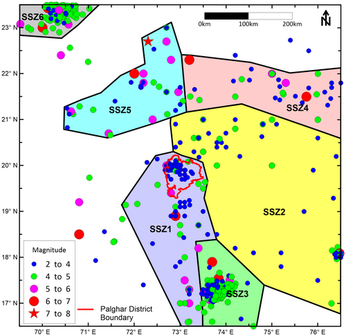
The area covering west coast is designated as SSZ1 which includes the Palghar district. The region covering the UGF, TNF, and part of Deccan Trap is considered as SSZ2 which includes the epicenter of $M_{W}$ 6.2 magnitude Killari earthquake of September 29, 1993. The Koyna region is taken as SSZ3 which includes $M_{W}$ 6.4 magnitude Koyna earthquake of December 10, 1967. SSZ4 represents the SONATA rift zone, SSZ5 falls under the Sourashtra region and SSZ6 falls under the Kutch region.

3.3 Completeness of the Catalogue

It is understood that old, low-magnitude earthquakes with insufficient instrumentation often have incomplete data in the catalog. The occurrence rates of these events can be assessed using recent data, specifically spanning the last

25

years, because of their short return periods. But the data for a longer period must be taken into account to have a reliable estimate for the occurrence rates of large magnitude earthquakes. The mean rates of earthquake occurrence may be underestimated if the data is not corrected for incompleteness. Finding the time period of complete data for a pre-set magnitude range will allow for the correction effectively. The entire set of data can then be used to calculate reliable mean earthquake occurrence rates for the specified magnitude ranges. The statistical method that Stepp [43] proposed to compute the completeness period is used in the current analysis. According to Stepp [43], earthquakes will obey a Poissonian distribution with a constant occurrence rates if all of the events are reported in a catalogue. For a time period of T years, if

E (M)

is the annual average number of events for a particular magnitude interval centered about

M

, the standard deviation

S_{E}

E (M)

is given by

S_{E} = \sqrt{E (M) / T}

()

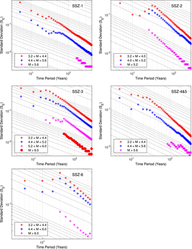
The stationarity of $E (M)$ ensures that $S_{E}$ behaves as $1 / \sqrt{T}$ . A significant departure of the $S_{E}$ values from the linearity of the $1 / \sqrt{T}$ slope yields the period of completeness (PoC) from the plot of $S_{E}$ versus $1 / \sqrt{T}$ , also referred to as the “completeness plot.” As the magnitude range increases, the PoC gets progressively longer. The completeness plots for all the SSZs are shown in Figure 4. The key results obtained from completeness analysis are summarized in Table 3.

Table 3. Estimated seismicity parameters for all the polygonal SSZs.

SSZ(s)	$b$ -value(s)	$a$ -value(s)	$M_{\max}$	$M_{\max}^{obs}$	Magnitude—PoC (in years)
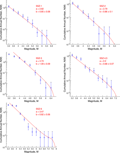
1	0.85 $\pm$ 0.08	2.82	7.04 $\pm$ 0.58	6.51	3.2–30, 4.4–40, 5.6–165
2	0.86 $\pm$ 0.10	2.79	6.65 $\pm$ 0.51	6.20	3.2–30, 4.0–70, 5.2–165
3	1.09 $\pm$ 0.09	4.73	6.59 $\pm$ 0.31	6.40	3.2–20, 4.4–50, 5.6–120, 6.0–255
4 + 5	0.68 $\pm$ 0.07	2.20	7.44 $\pm$ 0.50	7.01	3.2–30, 4.4–105, 5.6–180
6	0.82 $\pm$ 0.06	3.47	7.96 $\pm$ 1.29	7.70	3.2–20, 4.4–60, 6.0–150

3.4 Determination of $M_{\max}$

The highest seismic event that is typical of a region under seismotectonic and geological conditions is known as the maximum earthquake (

M_{\max}

). There are several techniques for figuring out

M_{\max}

values [44-46] and each technique always carries some subjectivity [47]. For instance, the Wells and Coppersmith [44] method requires the fault rupture length of upcoming earthquakes to be specified, but there is insufficient scientific evidence to make this determination with any degree of confidence. The Kijko–Sellevoll–Bayesian (KSB) method, a maximum likelihood method for maximum earthquake estimation, has been used in this study due to its broad acceptance and strong mathematical foundation. The Bayesian version of the Kijko–Sellevoll (KS) estimator of

M_{\max}

[48] can be constructed using knowledge of the Gutenberg–Richter (GR) probability distribution function (PDF), and the KSB estimator of

M_{\max}

can be computed through an iterative process. If

M_{\max}^{obs}

is the largest observed magnitude, the generic equation for

M_{\max}

prescribed by Kijko [48] is given by

M_{\max} = M_{\max}^{obs} + \int_{M_{\min}}^{M_{\max}} {[F_{M} (m)]}^{n} dm

()

where

F_{M} (m)

is the cumulative distribution function (CDF) and

n

is the number of events. In Equation (2),

M_{\max}

appears on both sides of the equation and hence an iterative method is followed to find an estimate of

M_{\max}

. The detailed procedure of finding

M_{\max}

by KSB method is given in this reference [48]. In the present analysis, the Matlab code developed by Kijko is used to compute

M_{\max}

for each SSZ.

3.5 Determination of Seismicity Parameters

When estimating seismic hazards, the assessment of seismicity parameters is thought to be the most crucial step. It is widely acknowledged that the frequency of earthquakes obeys an exponential distribution worldwide, indicated by Gutenberg and Richter [49] as

\log N (M) = a - bM

()

where

N (M)

is the cumulative number of events with magnitude equal to or greater than M. The mean annual number of earthquakes with a magnitude of zero or higher is

1 0^{a}

, and the relative likelihood of large and small earthquakes is represented by

b

(or the

b

value). Regression analysis is typically used to estimate the

a

and the

b

values from data that is available for a SSZ of interest. The standard Gutenberg–Richter (GR) relation holds good from

- \infty

+ \infty

in magnitude range. The impact of minor earthquakes are negligible for engineering purposes, and is generally ignored as it does not cause any significant damage [2]. As a result, it is required to set a lower bound, or to take into account a lower threshold (

M_{\min}

) on the magnitude. All SSZs, however, are always associated with a maximum magnitude (

M_{\max}

) or upper bound magnitude. The GR law then takes the form of a truncated exponential distribution by imposing a lower and an upper bound magnitude, in the magnitude range of

M_{\min}

M_{\max}

and is represented by [50]

N (M) = N (M_{\min}) \frac{e^{- β (M - M_{\min})} - e^{- β (M_{\max} - M_{\min})}}{1 - e^{- β (M_{\max} - M_{\min})}} M_{\min} < M < M_{\max}

()

A suitable $M_{\min}$ is required for the computation of hazard [51] even though the choice of $M_{\min}$ in Equation (4) is not crucial. $M_{\min}$ for this study is considered as $3.2$ and $β = b \ln 10$ . Using Weichert's [52] maximum likelihood method, the GR relationship for a SSZ is fitted by first determining the periods of completeness for various magnitude intervals. Due to the extremely low number of events in SSZs $4$ and $5$ , they are combined to provide a good fit for the truncated GR law. The magnitude-frequency dependence of SSZ $6$ is not well represented by exponential distribution of the truncated GR law of Equation (4). As a result, for this SSZ, a more intricate recurrence law called the characteristic earthquake recurrence law, invoked by Youngs and Coppersmith [53], is used. The exponentially decaying recurrence model of Equation (4) describes the observed seismicity well in specific area type of sources. However, many individual faults are seen to generate repeatedly the maximum earthquakes in a narrow magnitude range with a much higher occurrence rate than that predicted by the recurrence relationship for smaller magnitudes on the same fault. This has led to the concept of characteristic earthquake model which describes the observed seismicity better due to recurrence model proposed by Youngs and Coppersmith [53]. Table 3 lists the seismicity parameters for each polygonal SSZ. Figure 5 displays the magnitude-frequency distribution curves for each SSZ.

3.6 Determination of Smooth-Gridded Seismicity

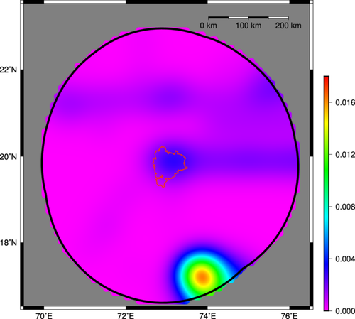
A physically plausible representation is not offered by the conventional uniform spatial distribution model of seismicity, also known as uniformly smoothed seismicity. The region under study shows distributed seismicity and Kernel-smoothed seismicity approach is the most accepted one as it is found to be a suitable alternative to account for the epistemic uncertainty in PSHA framework [54]. Therefore, the activity rates in each SSZ are determined using the smooth-gridded seismicity model [28]. The annual activity rates in the smooth-gridded seismicity are spatially varying, but the $M_{\max}$ and the $b$ -value stay constant within the source zones. According to this, there is no correlation between the $b$ -value and the activity rate, and the probability of earthquakes within a zone is not distributed uniformly [55]. Conversely, the uniform areal seismicity hypothesis states that there is an equal probability of earthquakes occurring at every point in the zone.

The discrete earthquake distributions can be modeled into spatially continuous probability distributions using the smooth-gridded seismicity model. In the current study, the method provided by Frankel [28] is used for this purpose. Several researchers have previously used this technique [9, 55-59]. The following is the smoothed function:

N_{i} (m_{r}) = \frac{\sum_{j} n_{j} {(m_{r}) e^{- (d_{ij} / c)}}^{2}}{{\sum_{j} e^{- (d_{ij} / c)}}^{2}}

()

where

c

indicates the correlation distance, which is related to the uncertainty in the epicentral location and is assumed to be

50

km in this analysis,

d_{ij}

is the distance between

ith

and

jth

cells, and

n_{j} (m_{r})

is the number of events with magnitude

\geq m_{r}

. The sum is computed in cells

j

within a distance of

3 c

of cell

i

. For threshold magnitude

3.2

M_{W}

, the annual activity rate

λ_{m_{r}}

is calculated as

N_{i} (m_{r}) / T

, where

T

is the (sub)catalogue period. The period of years

1990 - 2021

are covered by the sub-catalogue for the threshold magnitude of

3.2

M_{W}

. Figure 6 shows the smoothened annual activity rate for threshold magnitude

3.2

M_{W}

. It is possible to identify the areas of expected asperities using the smooth-gridded seismicity analysis [9].

3.7 Data-Driven Methods for Suitability Check of GMPEs

Selecting and prioritizing GMPEs based on recorded strong motion data is crucial for effectively applying the logic tree method in the PSHA to integrate epistemic uncertainties. A comprehensive and in-depth quantitative analysis has been conducted to determine the most appropriate GMPEs in the study area. To this end, 16 GMPEs were selected and their performance was compared to the observation (the strong motion data that was recorded). There are multiple approaches to assess the goodness-of-fit metrics [29, 60-62]. The Likelihood (LH) method is one of them which is a transparent one, based on the concept of likelihood [63]. However, the LH method is subject to certain subjectivities, even though it is statistically significant. Its effectiveness depends on the sample size, or the total amount of strong motion data that have been recorded. Subjectivities are found in the definition of ranks and in the threshold values of the goodness-of-fit measures. Scherbaum et al. [29] suggested the LLH method, a different goodness-of-fit technique that is independent of ad hoc assumptions, to get around these drawbacks.

Information theory ideas serve as the foundation for the LLH approach. Measuring the Kullback–Leibler (KL) distance between two models—a model that represents reality (in this case, the ground motion data) and a candidate ground motion model (in this case, a GMPE) is the main goal of the LLH method. When two probability density functions,

f (x)

and

g (x)

, describe two models,

f

and

g

, the KL distance between them is expressed as [29]

D (f, g) = E_{f} [\log_{2} (f)] - E_{f} [\log_{2} (g)]

()

where

E_{f}

statistical expectation of the LLH of the model function with respect to

f

D (f, g)

denotes the amount of information lost if model

f

is replaced by model

g

and is understood as the relative entropy between

f

and

g

[64]. A natural distance measure is indicated by a negative value of the statistical expectation [29] of the LLH function. The relative KL distance is the only measure that matters when comparing models because the statistical expectation of the LLH of

f

with respect to

f

cancels out as a constant term [29]. The LLH score can therefore be defined as follows to define a ranking criterion:

LLH = - \frac{1}{N} \sum_{n = i}^{N} \log_{2} (g (x_{i}))

()

N

is the total number of observations in this case. This LLH score is called average sample LLH. More explicitly, the LLH score in Equation (7) is expressed as

LLH = - \frac{1}{N} \sum_{n = i}^{N} \log_{2} [\frac{1}{σ_{i} \sqrt{2 π}} exp \{- \frac{1}{2} {(\frac{y_{i} - μ_{i}}{σ_{i}})}^{2}\}]

()

Here, the observed ground motion value is denoted by $y_{i}$ , and the mean and standard deviation of the GMPE under consideration are represented by $μ_{i}$ and $σ_{i}$ . A GMPE that performs better for a target region is indicated by a lower LLH score. With the LLH approach, a GMPE's suitability can be evaluated using just one metric - the LLH score, which essentially represents the average information loss that occurs when a candidate GMPE replaces the model that represents reality. On the other hand, the LH method requires the combination of four measures to determine the ranking criteria. Thus, the LLH approach is considered to be superior then LH approach.

3.8 Ground Motion Data Set

The region in which the study area is located has limited strong motion data available. A set of $66$ three-component strong-motion accelerograms ( $132$ horizontal accelerograms of longitudinal and transverse components) available from $53$ earthquakes have been considered to perform the suitability test of GMPEs. Out of these $53$ earthquakes, $51$ haven been reported in Koyna region, Maharashtra and the other two earthquakes took place at Bhuj, Gujarat and at Osmanabad, Maharashtra. The Bhuj earthquake (January 26, 2001) was recorded at Ahmedabad Station, Gujarat and all other earthquakes were recorded at Koyna Dam (Shear Zone Gallery, 1A Gallery, 1B Gallery, Koyna Dam Downstream, Koyna Dam Top, Kirnos Observatory, Middle Gallery and Koyna Dam Bottom). The earthquakes considered are listed in Table 4. The strong-motion data, used for performing the efficacy test of GMPEs, have been taken from the records available at Central Water and Power Research Station (CWPRS), Pune and few have been downloaded from Center for Engineering Strong Motion Data.

Table 4. List of earthquakes used for performing the suitability analysis.

Serial no.	Date (dd/mm/yy)	Lat ( $° N$ )	Lon ( $° E$ )	$M_{W}$	$H$ (km)	$R_{epi}$ (km)
1	12/09/1967	17.43	73.72	3.9	3.0	4.9
2	13/09/1967	17.40	73.70	4.5	5.0	5.5
3	13/09/1967	17.36	73.76	3.2	7.0	4.3
4	16/11/1967	17.45	73.85	3.5	8.0	12.0
5	10/12/1967	17.51	73.73	6.5	12.0	12.0
6	11/12/1967	17.30	73.89	3.8	8.0	18.5
7	12/12/1967	17.40	73.76	3.6	3.0	1.1
8	12/12/1967	17.28	73.69	4.7	13.0	14.1
9	13/12/1967	17.30	73.78	4.6	15.0	11.7
10	13/12/1967	17.49	73.78	3.8	23.0	9.8
11	14/12/1967	17.31	73.78	4.1	12.5	10.7
12	14/12/1967	17.37	73.75	4.1	5.0	3.0
13	17/12/1967	17.31	73.75	3.7	3.0	10.0
14	24/12/1967	17.35	73.71	5.0	20.0	6.9
15	24/12/1967	17.35	73.71	5.0	20.0	6.9
16	12/01/1968	17.39	73.75	4.1	4.0	1.5
17	12/01/1968	17.39	73.75	4.1	4.0	1.5
18	14/02/1968	17.33	73.70	3.6	16.0	8.9
19	04/03/1968	17.36	73.77	4.2	10.0	4.0
20	04/03/1968	17.36	73.77	4.2	10.0	4.0
21	29/10/1968	17.35	73.72	5.2	6.5	6.0
22	29/10/1968	17.35	73.72	5.2	6.5	6.0
23	29/10/1968	17.35	73.72	5.2	6.5	6.0
24	27/06/1969	17.40	73.74	3.9	3.0	1.8
25	27/06/1969	17.40	73.74	4.7	3.0	1.1
26	01/01/1970	17.33	73.71	4.3	11.0	9.0
27	27/05/1970	17.48	73.81	4.4	3.0	9.0
28	17/06/1970	17.32	73.31	3.6	1.0	49.1
29	17/06/1970	17.32	73.31	3.6	1.0	49.1
30	26/09/1970	17.37	73.65	4.4	13.0	11.0
31	14/02/1971	17.36	73.83	4.2	3.0	9.0
32	17/02/1974	17.25	73.76	4.7	19.0	16.0
33	29/05/1974	17.49	73.78	3.5	11.0	11.0
34	29/07/1974	17.32	73.75	4.3	24.0	8.0
35	02/09/1975	17.36	73.69	4.0	7.0	8.0
36	14/03/1976	17.24	73.73	3.9	5.0	18.0
37	22/04/1976	17.36	73.68	3.8	13.0	9.0
38	12/12/1976	17.38	73.73	3.9	13.0	3.0
39	19/09/1977	17.27	73.75	4.0	19.0	13.0
40	02/09/1980	17.24	73.74	4.3	6.0	17.5
41	02/09/1980	17.24	73.74	4.3	6.0	17.5
42	20/09/1980	17.21	73.76	4.7	8.0	21.0
43	20/09/1980	17.25	73.70	4.9	8.0	17.0
44	20/09/1980	17.25	73.70	4.9	8.0	17.0
45	26/10/1980	17.25	73.74	3.7	13.0	16.0
46	25/01/1981	17.30	73.73	3.7	7.0	11.0
47	25/04/1982	17.24	73.70	4.3	13.0	18.0
48	25/04/1982	17.24	73.70	4.3	13.0	18.0
49	14/11/1984	17.24	73.78	4.4	8.0	18.0
50	14/11/1984	17.24	73.78	4.4	8.0	18.0
51	29/10/1989	17.32	73.77	4.0	4.0	9.0
52	18/08/1993	17.34	73.75	3.6	5.0	6.0
53	28/08/1993	17.21	73.73	4.9	12.0	21.0
54	28/08/1993	17.20	73.78	4.9	12.0	20.0
55	03/09/1993	17.21	73.75	4.7	14.0	21.0
56	29/09/1993	18.11	76.60	6.3	15.0	321.0
57	08/12/1993	17.17	73.72	5.1	10.0	26.0
58	08/12/1993	17.20	73.76	5.1	8.0	21.0
59	01/02/1994	17.31	73.72	5.4	12.0	10.0
60	12/03/1995	17.25	73.73	4.7	5.0	17.0
61	13/03/1995	17.22	73.72	4.4	5.0	19.0
62	25/04/1997	17.35	73.76	4.4	3.0	6.0
63	12/03/2000	17.20	73.72	5.2	12.0	22.0
64	09/05/2000	17.17	73.76	3.9	2.0	25.0
65	10/09/2000	17.21	73.74	3.9	5.0	21.0
66	26/01/2001	23.42	70.23	7.7	16.0	239.0

3.9 GMPEs Used for Suitability Test

Since 2000, there has been a significant increase in seismic networks, leading to significant advancements in the development of GMPEs. The report by Douglas [65] provides a comprehensive and well-documented account of the empirical GMPEs that were in existence globally between 1964 and 2021. For the purpose of conducting the suitability test and ranking the GMPEs, 16 GMPEs developed for crustal earthquakes were primarily selected in accordance with the minimal criteria prescribed by Cotton et al. [26] and Bommer et al. [27]. The majority of the GMPEs are relatively robust, adequately constrained and latest. Twelve of the sixteen GMPEs were developed using the global data, and the other four, including one for the Himalayan region, were developed for other regions. Table 5 contains a list of all the GMPEs along with their range of applicability. It is important to note that India's small seismic network and lack of ground motion data make it difficult to develop reliable GMPEs through empirical means, at least not for the study areas. Additionally, it is added that, from the observation of Cotton et al. [26], a GMPE developed for a region that does not tectonically conform to the region under study should be excluded is not possibly correct because a GMPE can never be selected or excluded based on geographic criteria [27, 81]. With a few notable exceptions in active regions [82] for high-frequency response spectra, multiple studies demonstrate that there is no conclusive evidence of regional variations in ground motions in the regions of similar tectonic nature, at least from medium to large magnitude earthquakes [83, 84]. Instead, this criterion should be understood to mean that the GMPEs for subduction earthquakes should not be included in the hazard calculations for crustal earthquakes, and vice versa. For instance, GMPEs designed for volcanic areas should not be applied to areas that do not experience volcanic activity. As a result, the GMPEs shown in Table 5 have been taken into consideration for the target regions following the preliminary analysis.

Table 5. GMPEs used for suitability test with their range of applicability.

GMPEs with references	Magnitude ( $M_{W}$ ) range	Distance range (km)	$V_{s 30}$ range (m/s)	Periods (s)	Region
KAN06 [66]	5.5–8.2	$<$ 450	150–1500	0.0–5.0	Japan
ZHAO06 [67]	5–7.5	0–300	4 site classes	0.0–5.0	Japan
AS08 [68]	5–8.5	$<$ 200	$>$ 180	0.0–10	WW
BA08 [69]	5–8.0	0–200	180–1300	0.0–10	WW
CB08 [70]	4–8.5	0–200	150–1500	0.0–10	WW
CY08 [71]	4–8.5	0–200	150–1500	0.0–10	WW
IDR08 [72]	4.5–8	0–200	$>$ 450	0.0–10	WW
AKBO10 [73]	5–7.6	$<$ 100	3 site classes	0–3.0	MME
ASK14 [74]	3–8.5	0–300	180–1500	0.0–10	WW
BSSA14 [75]	3.0–8.5 (S, R) 3.3–7.0 (N)	0–400	150–1500	0.0–10	WW
CB14 [76]	3.3–8.5 (S) 3.3–8.0 (R) 3.3–7.0 (N)	0–300	150–1500	0.01–10	WW
CY14 [77]	3.5–8.5 (S) 3.5–8.0 (R, N)	0–300	180–1500	0.0–10	WW
IDR14 [78]	5–8.0	0–150	450–2000	0.0–10	WW
RKI07 [24]	5.0–8.0	30–300	4 site classes	0.0–4.0	Peninsular India
ZHAO16 [79]	5–7.5	0–300	4 site classes	0.0–5.0	WW
BJAN19 [80]	4–9.0	10–750	NA	0.0–10	Himalayas

Abbreviations: MME, Mediterranean, Middle East and Europe; N, normal; R, reverse; S, strike-slip; WW, world wide.

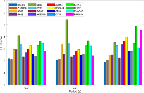
For ease of understanding and visualization, the bar diagrams of LLH scores at three relevant periods for PSHA for each of the GMPEs considered are shown in Figure 7. Because of their lowest LLH scores, Figure 7 makes it clear that the GMPEs developed by KAN06, ZHAO06, and IDR08 are the most appropriate for the current study region. It may be noted that GMPEs are developed by regression analysis to represent the functional form of recorded data. Mathematically, regression analysis means that once the functional form is developed, the GMPE model will extrapolate in a reasonable manner beyond the data range. Therefore, if the recorded data set used in the suitability analysis is not too far from the range of data set used for developing the GMPE, it is reasonable to use that GMPE. Consequently, to take care of the epistemic uncertainty, a combination of these three GMPEs with suitable weight factors has been chosen. The weight factors have been decided as per the prescription given in Scherbaum et al. [29]. Table 6 provides the LLH scores at the relevant periods as well as the weight factors assigned to each of these GMPEs. Each GMPE forms one branch of the logic tree. The construction of logic tree takes care of the epistemic uncertainty in PSHA formulation (here in terms of GMPEs).

Table 6. The LLH scores of the selected GMPEs at three periods of importance with respective weight factor.

GMPEs selected	0.01 s	LLH score 0.20 s	1.0 s	Weight factor
ZHAO06	2.11	2.05	2.06	0.36
KAN06	2.18	2.19	2.02	0.34
IDR08	2.35	2.24	2.20	0.30

It is added here that the study region falls in stable continental region (SCR). For SCR, strong motion data are limited and therefore SCR GMPEs are derived principally from the results of numerical simulations [85]. Therefore, it is found that the SCR GMPEs do not perform well in terms of LLH scores. For example, as mentioned in Section 2, the GMPE developed by Raghukanth and Iyenger [24] for SCR yields a higher LLH score compared to the other selected GMPEs. There are other issues with using SCR GMPEs. For example, Campbell [86] and Tavakoli and Pezeshk [87] used hard rock site conditions ( $V_{S 30}$ value∼2800 m/s) in their GMPEs but in our study, the seismic hazard is estimated at engineering bedrock (VS30 value 760 m/s). Therefore, in our study, we have selected 16 GMPEs primarily, based on the prescription of the minimum criteria proposed by Cotton et al. [26] and Bommer et al. [27]. Next, a data-driven approach for performing the efficacy test and the ranking of the GMPEs is carried away and finally three best performed GMPEs with appropriate weight factors, based on their LLH scores, have been chosen to do the analysis.

Recently, some authors [9, 88, 89] have carried away PSHA by constructing logic tree not only in terms of GMPEs, but also in terms of uncertainty in $b$ -value or the maximum expected magnitude. However, in the present analysis, the logic tree is constructed in terms of GMPEs only. Since our analysis is limited to a small district, the epistemic uncertainties arising out of the uncertainty in $b$ -value or the maximum expected magnitude are not likely to affect the final results notably.

3.10 Hazard Computation

Ground motion level is typically used to quantify the seismic hazard at a given location. The aggregate hazard at a specific location can be expressed by combining the seismic hazard values for each individual SSZ. The PSHA methodology takes into account the frequency with which the annual rate of ground motion at a given site of interest exceeds a given value for different return periods of the hazard. For a given possible earthquake magnitude at a source-to-site distance, the probability of exceeding a given value of $y^{*}$ of a ground motion parameter $Y$ is calculated, and it is then multiplied by the probability that the earthquake of that specific magnitude would occur at that specific location. After that, the procedure is repeated for every possible location and magnitude, with the probabilities of each being added up.

The total probability theorem [2] is used to calculate the probability that a ground motion parameter

Y

will exceed a specific value

y^{*}

for a given earthquake occurrence.

P [Y > y^{*}] = P [Y > y^{*} | X] P [X] = \int P [Y > y^{*} | X] f_{x} (X) d x

()

where

X

is a vector of random variables that influences

Y

. To compute the seismic hazard, the quantities in

X

are limited to magnitude (

M

) and distance (

R

). Assuming that

M

and

R

are independent, the PoE can be written as

P [Y > y^{*}] = \iint P [Y > y^{*} | m, r] f_{M} (m) f_{R} (r) d m d r

()

where

f_{M} (m)

and

f_{R} (r)

are the PDF and

P [Y > y^{*} | m, r]

is obtained from the predictive relationship for

M

and

R

respectively. While the site is in a region of

N_{s}

number of SSZs, and each SSZ has an average rate of threshold magnitude exceedance (or annual activity rate)

λ_{i}

, then, the total average exceedance rate for the region is given by

ν_{y^{*}} = \sum_{i}^{N_{s}} λ_{i} \iint P [Y > y^{*} | m, r] f_{M i} (m) f_{R i} (r) d m d r

()

For almost all realistic PSHAs, the integral 11 cannot be evaluated analytically. This means that numerical integration is necessary. The approach, generally employed, is to discretize the possible distance and magnitude ranges into

N_{M}

and

N_{R}

segments, respectively. Now, one can estimate the average exceedance rate by

ν_{y^{*}} = \sum_{i = 1}^{N_{s}} \sum_{j = 1}^{N_{M}} \sum_{k = 1}^{N_{R}} λ_{i} P [Y > y^{*} | m_{j}, r_{k}] f_{Mi} (m_{j}) f_{Ri} (r_{k}) Δ m Δ r

()

Assuming that each SSZ is able to produce

N_{M}

distinct earthquakes with a magnitude of

m_{j}

N_{R}

distinct source-to-site distances

r_{k}

, Equation (12) can take the form as

ν_{y^{*}} = \sum_{i = 1}^{N_{s}} \sum_{j = 1}^{N_{M}} \sum_{k = 1}^{N_{R}} λ_{i} P [Y > y^{*} | m_{j}, r_{k}] P [M = m_{j}] P [R = r_{k}]

()

The return period for the ground motion parameters

y^{*}

can be obtained by taking the reciprocal of

ν_{y^{*}}

. PSHA intends to generate a seismic hazard curve (SHC), which is represented as a plot of

ν_{y^{*}}

against

y^{*}

. The relationship between a ground motion parameter and its frequency of exceedance is provided by the SHC. The PoE of

y^{*}

in a finite time interval (say, for an exposure period

T

) can be estimated by combining the SHC with the Poisson model and is given by

P [Y_{T} > y^{*}] = 1 - e^{- ν_{y^{*}} T}

()

The PSHA computational method discussed above is applied to every grid point (site) at the engineering bedrock level ( $V_{S 30} \sim 760 m / s$ ). Using the framework provided by Kaklamanos et al. [90] for estimating unknown input parameters, the various distance parameters, such as rupture distance ( $R_{rup}$ ), horizontal distance to top edge of the rupture ( $R_{x}$ ), and so on, needed for implementing the GMPEs, have been determined.

4 Results and Discussion

At the engineering bedrock level conforming to $V_{S 30} = 760$ m/s, PGA and 5 $%$ damped PSA at 0.2 and 1.0 s for all the grid points for 10 $%$ and 2 $%$ PoE for a 50-year exposure period have been computed. The spatial distribution of the same, commonly known as seismic hazard maps, is shown in Figure 8 for MCE and DBE conditions (explained earlier). The left panel in Figure 8 shows the hazard maps for 475 years return period (DBE) while the right panel shows the same for 2475 years return period (MCE). For structural design purpose, 10 $%$ PoE in 50 years is regarded as more suitable. The spatial variation of PGA for 10 $%$ PoE in 50 years at engineering bed rock is in the range from 0.12 to 0.19 g for Palghar district. The PSA at 0.2 s shows a spatial variation between 0.28 and 0.47 g while for 1.0 s, it varies from 0.06 to 0.11 g. The PGA value for Palghar town has a hazard level to the tune of 0.16 g for DBE condition. Our present results significantly improve upon the deterministic zonation of BIS code [3] and captures the local variation in seismic hazard well, whereas BIS code [3] suggested to consider a uniform hazard value.

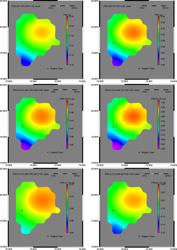
The spatial variation in PGA for 2 $%$ PoE in 50 years ranges from 0.21 to 0.31 g while PSA at 0.2 and 1.0 s shows a variation of 0.52–0.78 g and 0.13–0.20 g, respectively. The local variation in seismic hazard is evident from Figure 8. The consideration of nonuniform seismicity together with suitability test of GMPEs, based on extensive computation of quantitative assessment, has yielded an improved seismic hazard level for this region. The epistemic uncertainty is also taken care of by selecting three GMPEs with weight factors determined from the method provided by Scherbaum et al. [29].

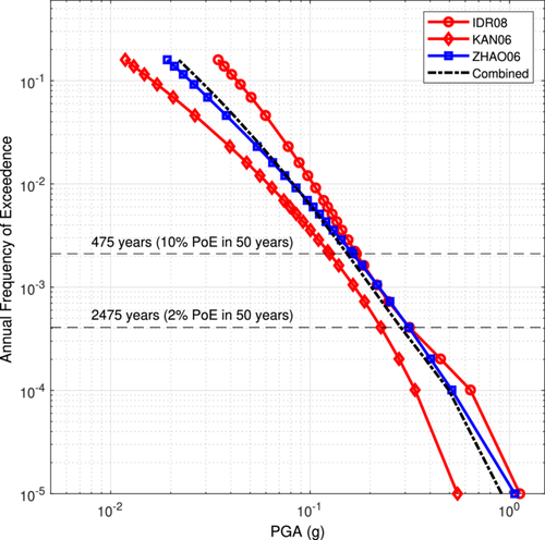
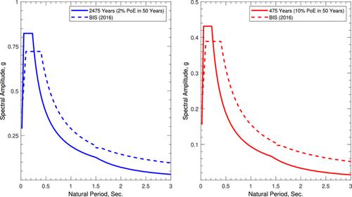
As defined in Subsection 3.10, the SHC is a graphic plot showing annual frequency of exceedance (AFE) against PGA or one of the PSAs. The SHC for the PGA at Palghar town for the three GMPEs selected are shown in Figure 9 together with the hazard curve obtained by combining the GMPEs with appropriate weight factors. The AFE values of 0.0021 and 0.000404 correspond to 10 $%$ and 2 $%$ probabilities of exceedance in 50 years, equivalent to 475 years and 2475 years of return periods, respectively. The SHC is also developed for PSA at 0.2 and 1 s at Palghar town (not shown here). The uniform hazard spectra (UHS) refers to a response spectrum with equal PoE in all the time periods. In PSHA, UHS are very important as these provide essential probabilistic information needed for an advanced seismic hazard analysis. UHS are also termed as target response spectra (TRS) from engineering perspective. The PGA and PSA values at 0.2 and 1 s are used to produce 5 $%$ damped TRS. The reason for selecting 0.2 and 1 s is already explained earlier. In this method, the local site condition is taken care of by various factors while calculating the control periods which mark the beginning of constant acceleration range and constant velocity range. The methodology of developing TRS by using spectral amplitude at selected periods is explained in the paper by Malhotra [32]. The comparison of 5 $%$ damped TRS at Palghar town for 10 $%$ and 2 $%$ PoE with that of BIS code [3] are plotted in Figure 10. It is noticed that the amplitudes of spectral acceleration obtained from BIS code [3] are on the lower side compared to those obtained from the present study for the natural periods 0.23 and 0.22 s for 10% and 2% PoE, respectively. The hazard curve and the $5 %$ damped TRS for any grid point (site) within the study area can be estimated from the hazard maps shown in Figure 8. From the 5 $%$ damped TRS, the acceleration time history, compatible with the TRS, and the design response spectra for any other value of damping can easily be computed [30]. The significance of the study lies in calculating the level of seismic hazard in a realistic way by considering the most suitable GMPEs in a region that hosts a number of dams and a nuclear power station. Since selection of GMPEs plays the most crucial role in PSHA, the hazard maps obtained from a combination of suitable GMPEs for this region makes the study relevant in designing new earthquake-resistant structures and evaluating seismic safety of existing structures. The outcome of the study will help in seismic microzonation for urban planning and land use management (Table 7).

Table 7. Horizontal component of ground motion values at the location of dams in Palghar district and TAPS.

Location	Lon (° $E$ )	Lat (° $N$ )	DBE (Horizontal) (g)			MCE (Horizontal) (g)
Location	Lon (° $E$ )	Lat (° $N$ )	PGA	PSA (0.2 s)	PSA (1.0 s)	PGA	PSA (0.2 s)	PSA (1.0 s)
TAPS	72.6617	19.8294	0.15	0.42	0.09	0.28	0.79	0.18
Dhamini	73.0608	19.9251	0.18	0.51	0.11	0.34	0.96	0.22
Kurze	72.9493	20.0757	0.17	0.47	0.10	0.32	0.94	0.21
Vandri	72.9539	19.6149	0.17	0.46	0.10	0.29	0.84	0.19
Vaitarna	73.2906	19.6708	0.17	0.48	0.10	0.32	0.93	0.21
Palghar Town	72.7699	19.6967	0.16	0.43	0.09	0.29	0.84	0.19

5 Conclusions

The purpose of the present research is to get the probabilistic seismic hazard map of Palghar district, Maharashtra, as the Palghar district has witnessed an unusual frequency of earthquakes recently. As the district houses an atomic power station and a number of dams, it is of extreme economical importance. Therefore, re-evaluation of seismic safety in terms of seismic hazard in a practical way for this region is very necessary. As the ground motion parameters are highly dependent on the choice of the GMPEs, it is indeed necessary to give due importance on the selection of appropriate GMPEs. The selection of GMPEs for a particular region from established methodology helps us to overcome the subjective judgment of choosing GMPEs. In the present work, following the minimum criteria proposed by Cotton et al. [26] and Bommer et al. [27], 16 GMPEs have been primarily selected for performing the efficacy test and ranking of the GMPEs. The suitability of these GMPEs is examined by performing a thorough quantitative assessment in a systematic way and finally three best performed GMPEs with appropriate weight factors, based on their LLH scores, have been used. Thus the present work has attempted to improve upon the previous works to some extent.

An updated and comprehensive earthquake catalogue, homogenized and declustered subsequently, has been employed in the present research. As the seismicity in Peninsular India is diffused in nature, smooth-gridded seismicity model is more appropriate than uniform areal seismicity model, as explained earlier. The hazard computations have been performed in a finer grid resolution of 0.02 $\times$ 0.02, which results in more accurate values of PGA and PSA. The probabilistic seismic hazard maps of Palghar district in engineering bed rock condition in terms of PGA and 5 $%$ damped PSA at 0.2 and 1.0 s for 475 years and 2475 years of return periods are presented. The hazard maps show considerable improvements over the previous studies, which is reflected in the spatial variation of the PGA and the PSA. The hazard curves and the TRS are also computed for Palghar town and the comparison of TRS with the BIS code [3] are shown. As PSHA is accepted to be the most rational means to quantify the seismic hazard [91], the present research focuses on developing seismic hazard maps in terms of PGA and PSA by following an advanced seismic design philosophy. Since a structure is expected to face all possibilities of occurrence of ground motion in its design life, the results, obtained from this PSHA study, can be used for designing and constructing earthquake-resistant structures in the area of the study, in addition to assessing seismic safety of the existing structures and serving for urban planning by identifying areas having different seismic hazard potential, known as microzonation. The values of PGA and 5 $%$ damped PSA at 0.2 and 1.0 s for some other important locations within the Palghar district, obtained from the present analysis, along with the same given in the Indian Standard [3] are shown in Table 8 for a comparison. It is observed that the values of PGA and 5 $%$ damped PSA at 1.0 s, obtained from our study is less than that of the Indian Standard [3] whereas the 5 $%$ damped PSA at 0.2 s appears higher than the Indian Standard. This finding is important because the natural periods of important structures generally lie around 0.2 s.

Table 8. Comparison of hazard level obtained from the present analysis with that of the Indian Standard [3].

Location	Lon (° $E$ )	Lat (° $N$ )	PGA (g)		PSA (0.2 s) (g)		PSA (1.0 s) (g)
Location	Lon (° $E$ )	Lat (° $N$ )	Indian standard	Present study	Indian standard	Present study	Indian standard	Present study
TAPS	72.6617	19.8294	0.20	0.15	0.32	0.42	0.17	0.10
Dhamini	73.0608	19.9251	0.24	0.18	0.46	0.51	0.20	0.12
Palghar Town	72.7699	19.6967	0.20	0.16	0.39	0.43	0.17	0.10
Vasai-East	72.8557	19.4056	0.17	0.13	0.32	0.35	0.14	0.09
Vasai-West	72.8155	19.3665	0.16	0.12	0.31	0.33	0.14	0.08
Boisar	72.7452	19.7969	0.20	0.16	0.39	0.43	0.17	0.10

Acknowledgments

S.S. gratefully acknowledges Prof. A.K. for providing the computer program for determination of $M_{\max}$ . The Generic Mapping Tools (GMT) software package [92] was used to prepare Figures 1, 6, and 8. The authors express their gratitude to Y.N.S., Additional Director, for his continuous support and encouragement. The authors are thankful to the anonymous reviewers for their useful comments which help the authors in improving the manuscript.

Conflicts of Interest

The authors declare no conflicts of interest.

References

1D. Srinagesh, D. K. Singh, G. Vikas, et al., “An Appraisal of Recent Earthquake Activity in Palghar Region, Maharashtra, India,” Current Science 118, no. 10 (2020): 1592.
10.18520/cs/v118/i10/1592-1598
Web of Science® Google Scholar
2S. L. Kramer, Geotechnical Earthquake Engineering (Pearson Education, Inc, 2013).
Google Scholar
3 BIS, “ Indian Standard Criteria for Earthquake Resistant Design of Structures,” in Part 1: General Provisions and Buildings, (Bureau of Indian Standards, 2016).
Google Scholar
4K. N. Khattri, “A Need to Review the Current Official Seismic Zoning Map of India,” Current Science 90 (2006): 634–636.
Web of Science® Google Scholar
5C. A. Cornell, “Engineering Seismic Risk Analysis,” Bulletin of the Seismological Society of America 58 (1968): 1583–1606.
10.1785/BSSA0580051583
Web of Science® Google Scholar
6R. K. McGuire, Fortran Computer Program for Seismic Risk Analysis, US Geological Survey, Open File Report (1976): 76–67.
Google Scholar
7S. Bhatia, M. R. Kumar, and H. K. Gupta, “A Probabilistic Seismic Hazard Map of India and Adjoining Regions,” Annali di Geofisica 42, no. 1 (1999): 153–166.
Google Scholar
8R. N. Iyengar, D. K. Paul, R. K. Bhandari, et al., Development of Probabilistic Seismic Hazard Map Probabilistic Seismic Hazard Map of India (Technical Report of the Working Committee of Experts Constituted by the National Disaster Management Authority, Government of India, 2011).
Google Scholar
9S. K. Maiti, S. K. Nath, M. D. Adhikari, N. Srivastava, P. Sengupta, and A. K. Gupta, “Probabilistic Seismic Hazard Model of West Bengal, India,” Journal of Earthquake Engineering 21 (2017): 1113–1157.
10.1080/13632469.2016.1210054
Web of Science® Google Scholar
10T. G. Sitaram, K. S. Vipin, and R. K. Ganesh, “A Study on Seismicity and Siesmic Hazards for the Karnataka State,” Journal of Earth System Sciences 121, no. 2 (2012): 475–490.
10.1007/s12040-012-0171-0
Google Scholar
11S. Kolathayar and T. G. Sitharam, “Characterization of Regional Seismic Source Zones in and Around India,” Seismological Research Letters 83, no. 1 (2012): 77–85.
10.1785/gssrl.83.1.77
Web of Science® Google Scholar
12B. Ghosh, J. W. Pappin, M. M. L. So, and K. M. O. Hicyilmaz, “Seismic Hazard Assessment of India,” in Proceedings of the Fifteenth World Conference on Earthquake Engineering, (Lisbon, Portugal 2012).
Google Scholar
13P. Anbazhagan, M. Sreenivas, B. Ketan, S. S. R. Moustafa, and N. S. N. Al-Arifi, “Selection of Ground Motion Prediction Equations for Seismic Hazard Analysis of Peninsular India,” Journal of Earthquake Engineering 20 (2016): 699–737.
10.1080/13632469.2015.1104747
Web of Science® Google Scholar
14K. Jaiswal and R. Sinha, “Probabilistic Seismic-Hazard Estimation for Peninsular India,” Bulletin of the Seismological Society of America 97, no. 1 (2007): 318–330.
10.1785/0120050127
Web of Science® Google Scholar
15L. Kanagarathinam, G. R. Dodagoudar, and A. Boominathan, “Probabilistic Seismic Hazard Studies of East Coast Region of India,” in Proceedings of the Fourteenth World Conference on Earthquake Engineering, (Beijing, China 2008).
Google Scholar
16P. Anbazhagan, J. S. Vinod, and T. G. Sitharam, “Probabilistic Seismic Hazard Analysis for Bangalore,” Natural Hazards 48 (2009): 145–166.
10.1007/s11069-008-9253-3
Web of Science® Google Scholar
17K. S. Vipin, P. Anbazhagan, and T. G. Sitharam, “Estimation of Peak Ground Acceleration and Spectral Acceleration for South India With Local Site Effects: Probabilistic Approach,” Natural Hazards and Earth System Sciences 9 (2009): 865–878.
10.5194/nhess-9-865-2009
Web of Science® Google Scholar
18A. D. Roshan and P. C. Basu, “Application of PSHA in Low Seismic Region: A Case Study on NPP Site in Peninsular India,” Nuclear Engineering and Design 240 (2010): 3443–3454.
10.1016/j.nucengdes.2010.04.037
CAS Web of Science® Google Scholar
19A. Menon, T. Ornthammarath, M. Corigliano, and C. G. Lai, “Probabilistic Seismic Hazard Macrozonation of Tamil Nadu in Southern India,” Bulletin of the Seismological Society of America 100, no. 1 (2010): 1320–1341.
10.1785/0120090071
Google Scholar
20P. Anbazhagan, P. Gajawada, and A. Parihar, “Seismic Hazard Map of Coimbatore Using Subsurface Fault Rupture,” Natural Hazards 60 (2012): 1325–1345.
10.1007/s11069-011-9915-4
Web of Science® Google Scholar
21T. G. Sitaram, K. S. Vipin, and R. K. Ganesh, “A Study on Seismicity and Siesmic Hazards for the Karnataka State,” Journal of Earth System Sciences 121, no. 2 (2012): 475–490.
10.1007/s12040-012-0171-0
Google Scholar
22A. C. Lindholm, I. A. Parvez, and D. Kühn, “Probabilistic Earthquake Hazard Assessment for Peninsular India,” Journal of Seismology 20 (2016): 629–653.
10.1007/s10950-015-9548-2
Web of Science® Google Scholar
23A. Scaria, I. D. Gupta, and V. K. Gupta, “An Improved Probabilistic Seismic Hazard Mapping of Peninsular Shield Region of India,” Soil Dynamics and Earthquake Engineering 141 (2021): 106417.
10.1016/j.soildyn.2020.106417
Web of Science® Google Scholar
24S. T. G. Raghu Kanth and R. N. Iyengar, “Estimation of Seismic Spectral Acceleration in Peninsular India,” Journal of Earth System Science 116 (2007): 199–214.
10.1007/s12040-007-0020-8
Web of Science® Google Scholar
25N. A. Abrahamson and W. J. Silva, “Empirical Response Spectral Attenuation Relations for Shallow Crustal Earthquakes,” Seismological Research Letters 68 (1997): 94–127.
10.1785/gssrl.68.1.94
Google Scholar
26F. Cotton, F. Scherbaum, J. J. Bommer, and H. Bungum, “Criteria for Selecting and Adjusting Ground-Motion Models for Specific Target Regions: Application to Central Europe and Rock Sites,” Journal of Seismology 10 (2006): 137–156.
10.1007/s10950-005-9006-7
Web of Science® Google Scholar
27J. J. Bommer, J. Douglas, F. Scherbaum, F. Cotton, H. Bungum, and D. Fah, “On the Selection of Ground-Motion Prediction Equations for Seismic Hazard Analysis,” Seismological Research Letters 81 (2010): 783–793.
10.1785/gssrl.81.5.783
Web of Science® Google Scholar
28A. Frankel, “Mapping Seismic Hazard in the Central and Eastern United States,” Seismological Research Letters 66, no. 4 (1995): 8–21.
10.1785/gssrl.66.4.8
Google Scholar
29F. Scherbaum, E. Delavaud, and C. Riggelsen, “Model Selection in Seismic Hazard Analysis: An Information-Theoretic Perspective,” Bulletin of the Seismological Society of America 99 (2009): 3234–3247.
10.1785/0120080347
Web of Science® Google Scholar
30 ASCE, Minimum Design Loads for Buildings and Other Structures (American Society of Civil Engineers, 2010).
Google Scholar
31 ICC, Country Club Hills, Illinois (International Code Council, Inc, 2009).
Google Scholar
32P. K. Malhotra, “Smooth Spectra of Horizontal and Vertical Ground Motions,” Bulletin of the Seismological Society of America 96, no. 2 (2006): 506–518.
10.1785/0120050062
Web of Science® Google Scholar
33S. Dasgupta, P. Pande, D. Ganguly, et al., Seismotectonic Atlas of India and Its Environs (Geological Survey of India, 2000).
Google Scholar
34K. Jaiswal and R. Sinha, “Webpotral on Earthquake Disaster Awareness in India,” (2004), http//www.eatrhquakeinfo.org.
Google Scholar
35T. Oldham, “A Catalogue of Indian Earthquakes From the Earliest Time to the End of A. D. 1869,” Memoirs of the Geological Survey of India 1883 (1869): 163–215.
Google Scholar
36A. N. Tondon and H. M. Chaudhury, Koyna Earthquake of December, Scientific Report No. 59 (India Meteorology Department, 1968).
Google Scholar
37B. R. Rao and P. S. Rao, “Historical Seismicity of Peninsular India,” Bulletin of the Seismological Society of America 74, no. 6 (1984): 2519–2533.
10.1785/BSSA0740062519
Web of Science® Google Scholar
38K. T. Filiz and R. F. Kartal, “The New Empirical Magnitude Conversion Relations Using an Improved Earthquake Catalogue for Turkey and Its Near Vicinity (1900–2012),” Turkish Journal of Earth Sciences 25 (2012): 300–310.
Google Scholar
39E. M. Scordilis, “Empirical Global Relations Converting MS and MB to Moment Magnitude,” Journal of Seismology 10 (2006): 225–236.
10.1007/s10950-006-9012-4
Web of Science® Google Scholar
40S. A. Sipkin, “A Correction to Body-Wave Magnitude MB Based on Moment Magnitude MW,” Seismological Research Letters 74, no. 6 (2003): 739–742.
10.1785/gssrl.74.6.739
Google Scholar
41T. H. Heaton, F. Tajima, and A. W. Mori, “Estimating Ground Motions Using Recorded Accelerograms,” Surveys in Geophysics 8 (1986): 25–83.
10.1007/BF01904051
Web of Science® Google Scholar
42R. Uhrhammer, “Characteristics of Northern and Central California Seismicity,” Earthquake Notes 57, no. 21 (1986): 9.
Google Scholar
43J. C. Stepp, “Analysis of Completeness of the Earthquake Sample in the Puget Sound Area and Its Effects on Statistical Estimate of Earthquake Hazard,” in Proceedings of the International Conference on Microzonation for Safer Construction Research and Application (1972): 897–910.
Google Scholar
44D. L. Wells and K. J. Coppersmith, “New Empirical Relationships Among Magnitude, Rupture Length, Rupture Width, Rupture Area, and Surface Displacement,” Bulletin of the Seismological Society of America 84, no. 4 (1994): 974–1002.
10.1785/BSSA0840040974
Web of Science® Google Scholar
45A. Kijko, “Estimation of the Maximum Earthquake Magnitude,” Pure and Applied Geophysics 161 (2004): 1655–1681.
10.1007/s00024-004-2531-4
Web of Science® Google Scholar
46A. Kijko and G. Graham, “Parametric-Historic Procedure for Probabilistic Seismic Hazard Analysis Part I: Estimation of Maximum Regional Magnitude M Max,” Pure and Applied Geophysics 152 (1998): 413–442.
10.1007/s000240050161
Web of Science® Google Scholar
47G. A. Bollinger, M. S. Sibol, and M. C. Chapman, “Maximum Magnitude Estimation for an Intraplate Setting—Example: The Giles County, Virginia, Seismic Zone,” Seismological Research Letters 63, no. 2 (1992): 139–152.
10.1785/gssrl.63.2.139
Google Scholar
48A. Kijko and M. Singh, “Statistical Tools for Maximum Possible Earthquake Magnitude Estimation,” Acta Geophysica 59, no. 4 (2011): 674–700.
10.2478/s11600-011-0012-6
Web of Science® Google Scholar
49B. Gutenberg and C. F. Richter, “Frequency of Earthquakes in California,” Bulletin of the Seismological Society of America 34 (1944): 185–188.
10.1785/BSSA0340040185
Google Scholar
50C. A. Cornell and H. E. Vanmarcke, “The Major Infuence on Seismic Risk,” in Proceedings of the Fourth World Conference on Earthquake Engineering, Santiago, Chile (1969): 69–93.
Google Scholar
51J. J. Bommer and H. Crowley, “The Purpose and Definition of the Minimum Magnitude Limit in PSHA Calculations,” Seismological Research Letters 88, no. 4 (2017): 1097–1106.
10.1785/0220170015
Web of Science® Google Scholar
52D. H. Weichert, “Estimation of the Earthquake Recurrence Parameters for Unequal Observation Periods for Different Magnitudes,” Bulletin of the Seismological Society of America 70, no. 4 (1980): 1337–1346.
10.1785/BSSA0700041337
Web of Science® Google Scholar
53R. R. Youngs and K. J. Coppersmith, “Implication of Fault Slip Rates and Earthquake Recurrence Models to Probabilistic Seismic Hazard Estimates,” Bulletin of the Seismological Society of America 75, no. 4 (1985): 939–964.
Google Scholar
54J. Dhanya, K. P. Sreejaya, and S. T. G. Raghukanth, “Seismic Recurrence Parameters for India and Adjoined Regions,” Journal of Seismology 26 (2022): 1051–1075.
10.1007/s10950-022-10093-w
Web of Science® Google Scholar
55S. K. Nath and K. K. S. Thingbaijam, “Probabilistic Seismic Hazard Assessment of India,” Seismological Research Letters 83 (2012): 135–149.
10.1785/gssrl.83.1.135
Web of Science® Google Scholar
56A. D. Frankel, M. D. Petersen, C. S. Mueller, et al., “Documentation for the 2002 Update of National Seismic Hazards Maps,” U.S. Geological Survey Open File Report 2 (2002): 2–420.
Google Scholar
57M. W. Stirling, G. H. McVerry, and K. R. Berryman, “A New Seismic Hazard Model for New Zealand,” Bulletin of the Seismological Society of America 92 (2002): 1878–1903.
10.1785/0120010156
Web of Science® Google Scholar
58B. S. Motnikar and P. Zupancic, “Probabilistic Seismic Hazard Assessment Methodology for Distributed Seismicity,” Bulletin of the Seismological Society of America 93 (2003): 2502–2515.
10.1785/0120020182
Web of Science® Google Scholar
59K. Jaiswal and R. Sinha, “Probabilistic Seismic-Hazard Estimation for Peninsular India,” Bulletin of the Seismological Society of America 97 (2007): 318–330.
10.1785/0120050127
Web of Science® Google Scholar
60F. Scherbaum, F. Cotton, and P. Smit, “On the Use of Response Spectral-Reference Data for the Selection and Ranking of Ground-Motion Models for Seismic-Hazard Analysis in Regions of Moderate Seismicity: The Case of Rock Motion,” Bulletin of the Seismological Society of America 94 (2004): 2164–2185.
10.1785/0120030147
Web of Science® Google Scholar
61O. Kale and S. Akkar, “A New Procedure for Selecting and Ranking Ground-Motion Prediction Equations (GMPEs): The Euclidean Distance-Based Ranking (EDR) Method,” Bulletin of the Seismological Society of America 103 (2013): 1069–1084.
10.1785/0120120134
Web of Science® Google Scholar
62M. Kowsari, B. Halldorsson, B. Hrafnkelsson, and S. Jónsson, “Selection of Earthquake Ground Motion Models Using the Deviance Information Criterion,” Soil Dynamics and Earthquake Engineering 117 (2019): 288–299.
10.1016/j.soildyn.2018.11.014
Web of Science® Google Scholar
63A. W. F. Edwards, Likelihood, Expanded (Johns Hopkins University Press, 1992).
10.56021/9780801844454
Google Scholar
64T. M. Cover and J. A. Thomas, Elements of Information Theory, 2nd ed. (Wiley, 2006).
Google Scholar
65J. Douglas, “Ground Motion Prediction Equations 1964–2021,” 2022, http://www.gmpe.org.uk.
Google Scholar
66T. Kanno, “A New Attenuation Relation for Strong Ground Motion in Japan Based on Recorded Data,” Bulletin of the Seismological Society of America 96 (2006): 879–897.
10.1785/0120050138
Web of Science® Google Scholar
67J. X. Zhao, J. Zhang, A. Asano, et al., “Attenuation Relations of Strong Ground Motion in Japan Using Site Classification Based on Predominant Period,” Bulletin of the Seismological Society of America 96, no. 3 (2006): 898–913.
10.1785/0120050122
Web of Science® Google Scholar
68N. Abrahamson and W. Silva, “Summary of the Abrahamson & Silva NGA Ground-Motion Relations,” Earthquake Spectra 24 (2008): 67–97.
10.1193/1.2924360
Web of Science® Google Scholar
69D. M. Boore and G. M. Atkinson, “Ground-Motion Prediction Equations for the Average Horizontal Component of PGA, PGV, and 5%-Damped PSA at Spectral Periods Between 0.01 s and 10.0 s,” Earthquake Spectra 24 (2008): 99–138.
10.1193/1.2830434
Web of Science® Google Scholar
70K. W. Campbell and Y. Bozorgnia, “NGA Ground Motion Model for the Geometric Mean Horizontal Component of PGA, PGV, PGD and 5% Damped Linear Elastic Response Spectra for Periods Ranging From 0.01 to 10s,” Earthquake Spectra 24 (2008): 139–171.
10.1193/1.2857546
Web of Science® Google Scholar
71B. J. Chiou and R. R. Youngs, “An NGA Model for the Average Horizontal Component of Peak Ground Motion and Response Spectra,” Earthquake Spectra 24 (2008): 173–215.
10.1193/1.2894832
Web of Science® Google Scholar
72I. M. Idriss, “An NGA Empirical Model for Estimating the Horizontal Spectral Values Generated by Shallow Crustal Earthquakes,” Earthquake Spectra 24, no. 1 (2008): 217–242.
10.1193/1.2924362
Web of Science® Google Scholar
73S. Akkar and J. J. Bommer, “Empirical Equations for the Prediction of PGA, PGV, and Spectral Accelerations in Europe, the Mediterranean Region, and the Middle East,” Seismological Research Letters 81, no. 2 (2010): 195–206.
10.1785/gssrl.81.2.195
Web of Science® Google Scholar
74N. A. Abrahamson, W. J. Silva, and R. Kamai, “Summary of the ASK14 Ground Motion Relation for Active Crustal Regions,” Earthquake Spectra 30, no. 3 (2014): 1025–1055.
10.1193/070913EQS198M
Web of Science® Google Scholar
75D. M. Boore, J. P. Stewart, E. Seyhan, and G. M. Atkinson, “NGA-West2 Equations for Predicting PGA, PGV, and 5% Damped PSA for Shallow Crustal Earthquakes,” Earthquake Spectra 30, no. 3 (2014): 1057–1085.
10.1193/070113EQS184M
Web of Science® Google Scholar
76K. W. Campbell and Y. Bozorgnia, “NGA-West2 Ground Motion Model for the Average Horizontal Components of PGA, PGV, and 5% Damped Linear Acceleration Response Spectra,” Earthquake Spectra 30, no. 3 (2014): 1087–1115.
10.1193/062913EQS175M
Web of Science® Google Scholar
77B. S. J. Chiou and R. R. Youngs, “Update of the Chiou and Youngs NGA Model for the Average Horizontal Component of Peak Ground Motion and Response Spectra,” Earthquake Spectra 30, no. 3 (2014): 1117–1153.
10.1193/072813EQS219M
Web of Science® Google Scholar
78I. M. Idriss, “An NGA-West2 Empirical Model for Estimating the Horizontal Spectral Values Generated by Shallow Crustal Earthquakes,” Earthquake Spectra 30, no. 3 (2014): 1155–1177.
10.1193/070613EQS195M
Web of Science® Google Scholar
79J. X. Zhao, S. Zhou, J. Zhou, et al., “Ground-Motion Prediction Equations for Shallow Crustal and Upper Mantle Earthquakes in Japan Using Site Class and Simple Geometric Attenuation Functions,” Bulletin of the Seismological Society of America 106 (2016): 1552–1569.
10.1785/0120150063
Web of Science® Google Scholar
80K. Bajaj and P. Anbazhagan, “Regional Stochastic GMPE With Available Recorded Data for Active Region's Application to the Himalayan Region,” Soil Dynamics and Earthquake Engineering 126 (2019): 105825.
10.1016/j.soildyn.2019.105825
Web of Science® Google Scholar
81V. V. Bykova, “On the Selection of Ground-Motion Prediction Equations During the Assessment of Seismic Hazard in Stable Continental Regions,” Seismic Instruments 52 (2016): 135–143.
10.3103/S074792391602002X
Google Scholar
82F. O. Strasser, N. A. Abrahamson, and J. J. Bommer, “Sigma: Issues, Insights and Challenges,” Seismological Research Letters 80 (2009): 40–56.
10.1785/gssrl.80.1.40
Web of Science® Google Scholar
83P. J. Stafford, F. O. Strasser, and J. J. Bommer, “An Evaluation of the Applicability of the NGA Models to Ground-Motion Prediction in the Euro-Mediterranean Region,” Bulletin of Earthquake Engineering 6 (2008): 149–177.
10.1007/s10518-007-9053-2
Web of Science® Google Scholar
84J. Douglas, “On the Regional Dependence of Earthquake Response Spectra,” ISET Journal of Earthquake Technology 44 (2007): 71–99.
Google Scholar
85J. P. Stewart, J. Douglas, M. Javanbarg, et al., “Estimation of Peak Ground Acceleration and Spectral Acceleration for the Global Earthquake Model,” Earthquake Spectra 31, no. 1 (2015): 19–45.
Google Scholar
86K. W. Campbell, “Prediction of Strong Ground Motion Using the Hybrid Empirical Method and Its Use in the Development of Ground Motion (Attenuation) Relations in Eastern North America,” Bulletin of the Seismological Society of America 93 (2003): 1012–1033.
10.1785/0120020002
Web of Science® Google Scholar
87B. Tavakoli, “Empirical-Stochastic Ground Motion Prediction for Eastern North America,” Bulletin of the Seismological Society of America 95 (2005): 2283–2296.
10.1785/0120050030
Web of Science® Google Scholar
88M. Arfa, H. A. Awad, H. Abbas, J. A. Peláez, and R. Sawires, “Probabilistic Seismic Hazard Assessment of the Southwestern Region of Saudi Arabia,” Applied Sciences 14, no. 15 (2024): 6600.
10.3390/app14156600
CAS Google Scholar
89R. Sawires, J. A. Pelaez, R. E. Fat-Helbary, and H. A. Ibrahim, “Bulletin of the Seismological Society of America,” Applied Sciences 106 (2016): 788–801.
Google Scholar
90J. Kaklamanos, L. G. Baise, and D. M. Boore, “Estimating Unknown Input Parameters When Implementing the NGA Ground-Motion Prediction Equations in Engineering Practice,” Earthquake Spectra 27, no. 4 (2011): 1219–1235.
10.1193/1.3650372
Web of Science® Google Scholar
91K. R. Collins, Y. K. Wen, and D. A. Foutch, “Dual Level Seismic Design: A Reliability Based Methodology,” Earthquake Engineering & Structural Dynamics 25, no. 12 (1996): 1433–1467.
10.1002/(SICI)1096-9845(199612)25:12<1433::AID-EQE629>3.0.CO;2-M
Web of Science® Google Scholar
92P. Wessel, F. J. Luis, L. Uieda, et al., “The Generic Mapping Tools Version 6,” Geochemistry, Geophysics, Geosystems 20 (2019): 5556–5564.
10.1029/2019GC008515
Web of Science® Google Scholar

Volume4, Issue1

March 2025

Pages 76-96

Probabilistic Seismic Hazard Assessment of Palghar District, Maharashtra, India by Considering Spatially Nonuniform Seismicity

ABSTRACT

1 Introduction

2 Seismo-Tectonic Setup of the Area of Study

3 Methodology

3.1 Earthquake Catalogue

3.2 Demarcation of SSZ

3.3 Completeness of the Catalogue

3.4 Determination of $M_{\max}$

3.5 Determination of Seismicity Parameters

3.6 Determination of Smooth-Gridded Seismicity

3.7 Data-Driven Methods for Suitability Check of GMPEs

3.8 Ground Motion Data Set

3.9 GMPEs Used for Suitability Test

3.10 Hazard Computation

4 Results and Discussion

5 Conclusions

Acknowledgments

Conflicts of Interest

References

Figures

References

Information

About Wiley Online Library

Help & Support

Opportunities

Connect with Wiley

Probabilistic Seismic Hazard Assessment of Palghar District, Maharashtra, India by Considering Spatially Nonuniform Seismicity

ABSTRACT

1 Introduction

2 Seismo-Tectonic Setup of the Area of Study

3 Methodology

3.1 Earthquake Catalogue

3.2 Demarcation of SSZ

3.3 Completeness of the Catalogue

3.4 Determination of M max

3.5 Determination of Seismicity Parameters

3.6 Determination of Smooth-Gridded Seismicity

3.7 Data-Driven Methods for Suitability Check of GMPEs

3.8 Ground Motion Data Set

3.9 GMPEs Used for Suitability Test

3.10 Hazard Computation

4 Results and Discussion

5 Conclusions

Acknowledgments

Conflicts of Interest

References

Figures

References

Related

Information

3.4 Determination of $M_{\max}$