Source Apportionment and Geostatistics: An Outstanding Combination for Describing Metals Distribution in Soil

2.1 Investigation area, soil sampling, preparation, and analysis

The investigation area Unterwellenborn is located in the Free State of Thuringia in the central part of Germany. The iron- and steelworks in Unterwellenborn, now belonging to the Stahlwerk Thüringen GmbH (SWT), have a long tradition. Since 1872 iron and steel were produced. In the 1990s, the production was changed from pig iron production in blast furnace to an electric steel manufacturing plant (www.stahlwerk-thueringen.de). In the vicinity of the Stahlwerk Thüringen 60 soil samples were collected in an area of about 12 km² (see Fig. 1). The samples were taken on an irregular grid due to different anthropogenic interventions, for example, the newly built circuitous roads or residential areas. Buildings, streets, the railway, cultivated fields, industrial buildings, and even industrial monuments characterize this area. At each sampling point, five subsamples from the upper 0–20 cm layer under comparable conditions were taken, which were mixed to one composite soil sample. The soil samples were dried (105°C), homogenized, and passed through a 2-mm-sieve. Microwave digestion with aqua regia (21 mL 12 M HCl and 7 mL 15.8 M HNO₃) was performed according to EN 13346:2000 15. The digestion was performed twice with 0.5 g soil for each sampling point. Each solution was filled up to 100 mL with diluted HNO₃ (0.5 M) and the concentration of 15 elements was analyzed. The concentration of Cd, Co, Cr, Cu, Ni, Pb, and V was determined with the ICP-MS Elan 6000 (PerkinElmer) using multi-element standard and Rh as internal standard for the calibration 16. The As concentration was determined with the flow injection hydride generation AAS-5100 ZL (PerkinElmer) and the concentration of Ca, Fe, K, Mg, Mn, Na, and Zn with the flame-AAS-3110 (PerkinElmer). All elements were detected with concentrations above the detection limit, calculated according to the German DIN-standard 17 and the certified reference material IAEA/SOIL-7 18 was analyzed to verify the trueness (p = 95%) of the analytical method.

2.2 Basic principles of the applied chemometric methods

2.2.1 Data pre-treatment

Three different statistical methods were applied in this investigation: APCS-MLR, MCR-ALS, and geostatistics. Each method demands its own type of data. Whereas the data requires no pre-treatment for the application of geostatistics, the data must be autoscaled for the two other methods. The data were autoscaled according to Eq. 1 for APCS-MLR and according to Eq. 2 for MCR-ALS 19.

(1)

(2)

where z_ij is the autoscaled value of x_ij, s_j is the standard deviation of variable j, s the mean value of variable j, i is the index of the feature, and j is the index of the object.

2.2.2 Applied source apportionment methods

Source apportionment methods are well established in atmospheric deposition studies but rarely used in soil sciences. The purpose of these methods is to find (emission) sources, which influence the investigated area profoundly. Thereby, each source influences the behavior or distribution of only some of the examined elements or compounds. With the so-called source composition profiles we can present up to which amount the elements are characterized by each source. The other important result of source apportionment studies is the so-called source contribution profile. This presents the impact of the sources onto the different sampling points, respectively, investigation area.

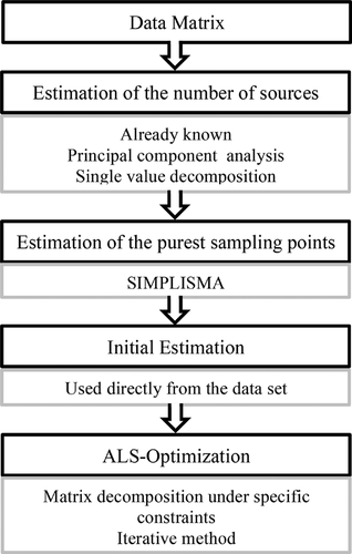
Performing a complete source apportionment survey of environmental data is a rather complicated task. Several steps must be carried out in order to achieve the composition and contribution profiles. Figures 2 and 3 present the flowcharts for the used methods APCS-MLR respectively MCR-ALS.

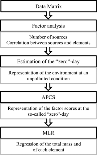
In order to find the hidden sources, a factor analysis must be performed to complete APCS-MLR. The factor analysis results in the number of sources and the correlation between the sources and elements. These results are used in the proceeding steps. In a perfect environmental condition no pollution would be occurring. This state presents the theoretical “zero”-day. It is also assumed, that sources only emit substances and, therefore, increase the pollution in the environment. With these considerations, the absolute principal component scores are calculated. In addition, the mass balance in order to accomplish APSC-MLR was needed. Then, a multiple linear regression between the APCS and the total mass was performed to obtain the source distribution profiles. Then, a multiple linear regression for each element was performed and the results were transformed into the source composition profiles.

Again, different steps must be done to accomplish MCR-ALS. First, the number of sources must be revealed. Common methods are principal component analysis or single value decomposition. If the number of sources is known, we have to select the proper sampling points. These have to represent each source specifically. These sampling points are used for the initial estimation and the alternating least squares algorithm is performed for the matrix decomposition. This results directly in the composition and distribution profiles.

The mathematical basis for both source apportionment methods is, as mentioned before, the decomposition of a data matrix into two smaller matrices and a residual matrix (Eq. 3).

(3)

where Z is the autoscaled data matrix, L^T is the transposed factor loadings matrix, respectively, the source contribution, S is the factor scores matrix, respectively, the source composition, Q is the residual matrix, n is the number of objects i, m is the number of features j, and p is the number of factors, respectively, sources k.

The requirements of the matrix decomposition are different for each method. For APCS-MLR, the requirement is the orthogonality of the resulting factors 20. Even though this method is named after principal components analysis, actually we performed a factor analysis with an extraction of principal components. Therefore, the amount of the explained variance decreases with each extracted factor. The number of considered factors can be chosen either due to the eigenvalues above one or the communalities. We rotated the resulting factors with Varimax rotation to achieve an easier interpretation 21. Starting from these results, we calculated absolute principal components scores and with those we performed a multiple linear regression of the total mass (Eq. 4) and for every single element 20.

(4)

where M_i is the particle mass recording during observation i, ζ is the particle mass contribution, APCS_ki is the rotated APCS for component k at observation i, and p is the number of pollution sources k.

In contrast to the requirement of orthogonality, for MCR-ALS, the requirement is non-negativity for S and L^T 22, 23. The unexplained variance Q is also minimized. The number of sources respectively factors cannot be calculated directly with MCR-ALS. In advance, the number of sources with factor analysis was estimated. With the SIMPLISMA method, the so-called purest sampling points for these were calculated 24, 25. These purest sampling points represent the purest contribution profiles of the data set. These had to be estimated, because ALS is an iterative method. Starting values need to be given to implement it. They were taken directly from the data set. The ALS optimization is done according to Eqs. 5 and 6 22. The iterative optimization is performed until no further improvement is found.

(5)

(6)

where S⁺ is the pseudo inverse matrix of S, L^T+ is the pseudo inverse matrix of L^T, and Z* is used for an improved stability and equals Z-Q_nm.

The results for the matrix decomposition for both methods are similar but not identical due to the different constraints. We used the correlation coefficient (Eq. 7) and the root mean squared error of prediction (RMSEP) (Eq. 8) of the multiple linear regression to evaluate both models.

(7)

(8)

where x_obs,i is the observed variable for object i, s the mean value of the observed variable, x_pred,i is the predicted variable for object i, and s the mean value of the predicted variable.

2.2.3 Geostatistical methods

With geostatistical methods the spatial dependence of the data is analyzed 26. A visualization of the element content with isoline plots is possible. Therefore, we estimated the content at unsampled locations with inverse distance weighting. The inverse distance weighting estimation is calculated according to Eq. 9 27, 28.

(9)

where z*(x₀) is the estimate of the unknown value z(x_o), z(x_i) are the values at the known sampling points, and d²(x_i x₀) is the distance between the unknown and the known sampling points.

2.3 Software

Excel 2010 (Microsoft) was used for general calculations of the data matrix, STATISTICA 6.1 (StatSoft) for factor analysis and multiple linear regression of the APCS-MLR-models, and MATLAB 7.9.0.529 (R2009b) (The MathWorks) for Windows 7 for the calculation of SIMPLISMA (spectral-mva-toolbox), and the MCR-ALS-model (MCR-ALS-toolbox). The toolboxes MCR-ALS and spectral-mva were downloaded from the following websites: www.mcrals.info and www.mathworks.com/matlabcentral/fileexchange/15391-multivariate-analysis-and-preprocessing-of-spectral-data. Surfer 9 (Golden Software) was used to calculate and illustrate the isoline plots.

3.1 Source apportionment methods

In environmental studies pollution, sources are often unknown and must be revealed by statistical tools. Factor analysis uncovers these sources and must be carried out to accomplish APCS-MLR 29. The principal components extraction method was used and the resulting factor loadings were rotated with Varimax rotation 19. Six factors were extracted with communalities >0.8 for each element. Two factors were described by a single element each and are, therefore, feature-own factors. These elements (K and Na) were removed for the succeeding source apportionment modeling analysis. Thus, the source apportionment studies were accomplished with 13 remaining elements (As, Ca, Cd, Co, Cr, Cu, Fe, Mn, Mg, Ni, V, Pb, and Zn). Now, the factor analysis results in three eigenvalues >1. Another possibility for the selection of relevant factors uses communalities. The communalities of factor 4 are >0.8 for all elements (see Table 1). Using communalities also suggests four factors instead of three.

The amount of the explained variance increased from 86% using three factors to 94% using four factors. With three factors, the variances of the heavy metals cadmium, nickel, and zinc are described insufficiently. Therefore, it is necessary to use four factors for the succeeding computation of the source apportionment studies.

The first important result of the source apportionment study is the percentage of explained variance for each source. The variance for both models differs due to the different requirements for the matrix decomposition. Table 2 summarizes the explained variance for both methods.

The requirements for the MCR-ALS-method do not include orthogonality, respectively, independence of the sources. Hence, the variances overlap. In this case, the variances overlap for almost 30%. Both models show resemblance: The explained variance for the complete model is very similar. The order of the sources is also alike. Only the results for source 4 (waste dump) differ: While the APCS-MLR-model explains 19% of the variance, the MCR-ALS-model explains 33%. The methods describe the impact of the waste dump onto the examined area differently.

To evaluate the quality of both models, the correlation coefficient and the relative prediction errors for both methods are given in Table 3.

The quality parameters for both models are also very similar. Only for the complete model the results of MCR-ALS are slightly worse. The correlation coefficient is for all elements >0.9. The relative prediction error is below 25% for all elements except for calcium and manganese. These results are satisfactory for a real model. Therefore, both models are useful to describe the existing sources in the examined region.

After comparing the general results of both models, the sources need to be discussed in more detail. The summarized results for both models are listed in Table 4.

The grouping of the elements is very reasonable for all sources and enables a rational interpretation. Source 1 includes typical elements for steel production. Therefore, source 1 was interpreted as iron industry emissions. In source 2 calcium and magnesium are grouped together. They indicate an interpretation of this source as limestone. In this region, limestone exists geologically and is quarried since 1963 (www.tagebau-kamsdorf.de). Source 3 includes arsenic, cobalt, and copper. These elements have also a geogenic origin and characterize the so-called Red Mountain 30. This mountain is rich of asbolane – a cobalt enriched ore. Source 4 includes cadmium, lead, and zinc. These elements are also related to the iron industry, but they are not emitted by it. It is likely, that these elements are still being deposited on the waste dump. There is one important difference between both methods. The number of elements, which are not described sufficiently by either one of the sources, varies considerably.

For a substantial interpretation, the source composition profiles need further discussion (Fig. 4). The source composition profiles allow a closer look on elements instead on sources. The loadings of the MCR-ALS-model had to be normalized to unity 31 for a better comparability of the two models. Additionally, the negative amounts of the composition profiles were set to zero, because sources can only emit elements and cannot force them to disappear.

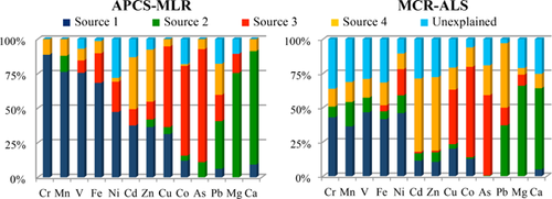
The source composition profiles differ remarkable, especially for sources 1 and 4. The most important difference is the high amount of unexplained variance for the MCR-ALS-model. Even though the loadings overlap due to the constraints in MCR-ALS, a lot of the variance is still unexplained. Another important difference is that the APCS-MLR-model assigns the elements more directly to one specific source instead of all existing ones. None of the elements is just characterized by one source. Usually three sources influence each element, sometimes even all four.

To complete the interpretation, the source contribution profiles for both models will be discussed (Figs. 5 and 6). The intensity of the source contribution profiles was normalized to compare the results of both models more easily.

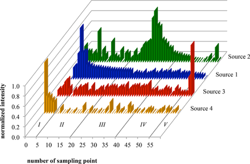
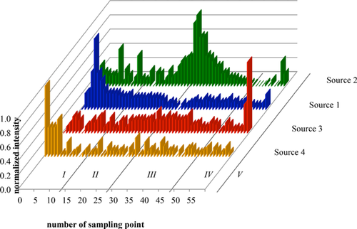
The source contribution profiles illustrated in Figs. 3 and 4 show a similar behavior for both methods. Source 1 influences mainly some sampling points (I + IV), source 2 a couple of sampling points (III), source 3 a few sampling points (V), and source 4 mainly one and partly up to five sampling points (I). These results also emphasize the interpretation of the sources. Source 2 is of geogenic origin, hence, a lot of sampling points are mainly influenced by this source. Source 4, however, is of anthropogenic origin and, therefore, characterizes only a few sampling points.

The results of both methods are similar. The main difference is the high amount of unexplained variance in the MCR-ALS-model. This can be seen as the weakness of this method. Even though the loadings overlap, a high amount (for some elements even up to 30%) of unexplained variance still exists. Furthermore, negative amounts for some elements for the source composition profiles appeared which would imply an element disappearance instead of emission. This is unrealistic for environmental studies. Elements are emitted from sources and do not vanish; especially in soil sciences because elements accumulate in soil.

3.2 Combination of geostatistics and source apportionment

It is possible to combine the results of the source contribution profiles with geostatistical methods. This can be done either for the results of MCR-ALS or APCS-MLR. Because the results of APCS-MLR are slightly better and can be used directly without further calculations, the distribution plots for this method are presented.

Therefore, the source-specific distribution of each element was interpolated. Altogether, 41 source-specific isoline plots out of 52 theoretical ones could be calculated. Because the sources do not influence all elements, there exist less isoline plots than theoretically could be expected. The source-specific element distribution plots illustrate very well the impact of each source onto the examined area. For example, in Fig. 7 the source-specific distribution of copper is illustrated.

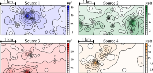
It is notable, that each source causes different hotspots. Source 1 has one big hotspot in the center of the area. Source 2 is responsible for hotspots in the eastern and western part of the region, source 3 in the southern part and the center and source 4 mainly in the southwestern part of the region. This implies that each source influences the region differently and the sources may influence the element distribution at more than one place.

The other source-specific element-distribution-plots are similar to the shown example in Fig. 5. This proves that the distribution caused by the sources is independent of the amount of emitted element. By considering not only the shape of each isoline plot but also the unit, a quantitative analysis is also possible. The impact of source 2 is about 18 μg/g at the hotspots and for source 3 up to 180 μg/g. This illustrates once more the results of the source apportionment. Source 3 characterizes the distribution of copper about 60% and source 2 only about 5%. In this case, the units of the source-specific isoline plots vary about one order of magnitude.

Another possibility to illustrate the source-specific distribution is to overlap them in one single plot. Figure 6 shows this overlapped source-specific distribution allowing a comprehensive interpretation.

The isoline plots illustrate the source-specific distribution very clearly (Fig. 8). Source 1 causes the main element distribution of chromium, iron, manganese, nickel, and vanadium. The hotspot of this source is located in the center of the region of interest. Samples in the immediate vicinity of the ironworks were taken, where the former iron industry smelter was located. Source 2 influences the distribution of calcium and magnesium. These elements have their highest contents where agricultural fields are located. They represent the limestone, which dominates this landscape. Source 3 characterizes the distribution of arsenic, cobalt, and copper. The highest content for these elements was found in the south of the examined area. At this point the so-called Red Mountain is located, where arsenic and copper enriched ore can be found 30. Source 4 describes mainly the distribution of cadmium, lead, and zinc. The highest content of these elements was found in the southwestern part of the examined area where the waste dump is situated. Furthermore, two smaller hotspots are near the source 1 hotspot. Without calculating the source-specific distribution, they would wrongly be linked to source 1 instead of source 3.

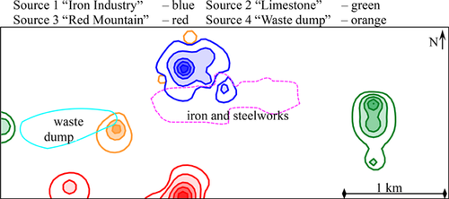
The visualization of the distribution of the elements confirms the results of the two source apportionment methods very well.

3.3 Advantages of the combination of receptor modeling methods with geostatistics

The combination of both methods can reveal hidden information. A clear distinction between different sources is possible. In addition, the elemental distributions caused by each source can be illustrated. Furthermore, the pattern of each source and the amount of emitted element could be visualized. The source description is quantitative and the impact of the source can be described very precisely. Therefore, the combination enables a reasonable interpretation of the data.