ORIGINAL ARTICLE

Full Access

Parameters affecting genome simulation for evaluating genomic selection method

Corresponding Author

Motohide Nishio

NARO Institute of Livestock and Grassland Science, Tsukuba, Japan

Correspondence: Motohide Nishio, NARO Institute of Livestock and Grassland Science, 2 Ikenodai, Tsukuba, Ibaraki 305-0901, Japan. (Email: [email protected])Search for more papers by this author

Masahiro Satoh,

Masahiro Satoh

NARO Institute of Livestock and Grassland Science, Tsukuba, Japan

Search for more papers by this author

Motohide Nishio,

Corresponding Author

Motohide Nishio

NARO Institute of Livestock and Grassland Science, Tsukuba, Japan

Correspondence: Motohide Nishio, NARO Institute of Livestock and Grassland Science, 2 Ikenodai, Tsukuba, Ibaraki 305-0901, Japan. (Email: [email protected])Search for more papers by this author

Masahiro Satoh,

Masahiro Satoh

NARO Institute of Livestock and Grassland Science, Tsukuba, Japan

Search for more papers by this author

First published: 19 May 2014

https://doi.org/10.1111/asj.12224

Citations: 2

Share a link

Email
Wechat
Bluesky

Abstract

The present study investigated the parameter settings for obtaining a simulated genome at steady state of allele frequency (mutation–drift equilibrium) and linkage disequilibrium (LD), and evaluated the impact of whether or not the simulated genome reached steady state of allele frequency and LD on the accuracy of genomic estimated breeding values (GEBVs). After 500 to 50 000 historical generations, the base population and subsequent seven generations were generated as recent populations. The allele frequency distribution of the last generations of the historical population and LD in the base population were calculated when varying the values of five parameters: initial minor allele frequency, mutation rate, effective population size, number of markers and chromosome length. The accuracies of GEBVs in the last generation of the recent population were calculated by genomic best linear unbiased prediction. The number of historical generations required to reach mutation–drift equilibrium depended on the initial allele frequency and mutation rate. Regardless of the parameters, LD reached a steady state before allele frequency distribution reached mutation–drift equilibrium. The accuracies of GEBVs largely reflect the extent of linkage disequilibrium with the exception of varying chromosome length, although there were no associations between the accuracies of GEBVs and allele frequency distribution.

Introduction

Advances in molecular biotechnology are making genome-wide high-density single nucleotide polymorphism (SNP) marker data available for livestock species. These data combined with phenotypic data can be used to calculate genomic estimated breeding values (GEBVs). This method was termed ‘genomic selection’ by Meuwissen et al. (2001). In their method, a Bayesian model is used to estimate thousands of marker effects simultaneously under the assumption that all quantitative trait loci (QTL) are in linkage disequilibrium (LD) with at least one marker. The GEBVs of all genotyped individuals in the population can then be calculated from the sum of all estimated marker effects. The expected advantage of this method over traditional selection methods are more accurate predictive ability (Daetwyler et al. 2008) and the potential to reduce inbreeding rates (Daetwyler et al. 2007; Dekkers 2007). Another approach for evaluating individuals without explicitly estimating marker effects is to estimate genomic relationships between individuals. These genomic relationships are used in the genomic best linear unbiased prediction (GBLUP) procedure, in which genomic relationships replace pedigree-based relationships in traditional BLUP (VanRaden 2008).

Many studies aim to increase the accuracy of GEBV; most use genome data generated by computer simulation. Simulation is a useful tool for assessing the performance of new algorithms and methods in genomic selection at very low cost and allows GEBVs to be compared with true genetic values. Simulations are basically carried out in two steps: (i) a historical population is simulated to reach steady state of allele frequency (mutation–drift equilibrium) and LD; (ii) a recent population is generated mimicking the livestock population, which can have a complex pedigree structure (Sargolzaei & Schenkel 2009). In this process, a large number of historical generations were required to establish a steady state allele frequency and LD. Thus, it is important to reduce a computational requirement by determining appropriate values of parameters for historical populations, such as mutation rate, effective population size and initial allele frequency in the historical generation, in particular when there are many numbers of loci and individuals. In previous simulation studies, there are no common criteria for determining such parameters Therefore, the accuracies of GEBVs obtained in previous studies may be affected not only by the performance of prediction methods, but also by whether or not simulated genome reaches steady state of allele frequency and LD.

The present study investigated the parameters affecting the number of generations in an historical population required to simulate a genome at steady state of allele frequency and LD and evaluated the impact of whether or not simulated genome reached steady state of allele frequency and LD on the accuracy of GEBV. Understanding these relationships will help simulating efficiently and fairly genome data to investigate the accuracy of GEBV. Here, the present study focused on GBLUP as a prediction method of GEBVs because GBLUP has become a popular approach in genomic sequencing (GS) of dairy cattle (McHugh et al. 2011; Wiggans et al. 2011).

Materials and Methods

Simulation data

An historical population was simulated for five numbers of generations (N_G = 500, 2000, 5000, 20 000, and 50 000) of random matings with an effective population size (N_e) of 100 (50 males and 50 females). The simulated genome consisted of one chromosome with a length (L) of 1 Morgan, containing 5000 randomly spaced SNP loci. The initial minor allele frequency (IMAF) of all SNPs was assumed to be 0, meaning all individuals were completely homozygous for the same allele in the first generation of the historical population. Mutation occured at a rate (u) of 10⁻⁴ per locus meiosis and involved the switching from one allele to another. Recombinations were sampled from a Poisson distribution with a mean of 1 per Morgan and were then randomly placed along the chromosome.

After N_G generations, a base population (G0) and the following seven generations (G1 to G7) were generated as the recent population. The size of G0 increased up to 400 (200 males and 200 females). In the following generations, 40 sires were randomly selected and mated to 200 dams in each generation. Each dam had one son and one daughter; thus, each sire had five sons and five daughters.

In G0, the numbers of SNP markers (N_m) and QTL (N_q) were 1000 and 100, respectively. These markers and QTL were randomly chosen from segregating SNP loci with a minor allele frequency > 0.01. The true breeding value was simulated by summing up all true QTL genotypic values, that is, $urn:x-wiley:13443941:media:asj12224:asj12224-math-5001$ , where m is the number of QTL; a_i is the allele substation effect of the i^th QTL; and W_i is 0, 1 or −1 corresponding to heterozygote, major and minor homozygote, respectively (Falconer & Mackay 1996). The allele substitution effects of QTL were drawn from a gamma distribution with a shape parameter of 0.42 and scale parameter of 1 (Meuwissen et al. 2001). The signs of allele substitution effects were drawn at random with equal chance. The total additive genetic variance ( $urn:x-wiley:13443941:media:asj12224:asj12224-math-5002$ ) was calculated as the sum of variances across all QTL, that is, 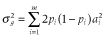$urn:x-wiley:13443941:media:asj12224:asj12224-math-5003$ , where p_i is the allele frequency at the i^th QTL. Trait heritability (h²) was set to 0.3. 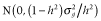To obtain phenotypic values, an environmental effect was added to the true breeding value, which was sampled from a normal distribution: $urn:x-wiley:13443941:media:asj12224:asj12224-math-5004$ .

The simulation process described above was defined as the base scenario (scenario 1). An additional five scenarios (scenarios 2 to 6) were defined using various values of IMAF (0.5), u(5.0 × 10⁻⁴), N_e (500), N_m (200) and L (5), respectively (Table 1). In scenario 6, the simulated genome consisted of one chromosome with a length of 5 Morgan, and N_m and N_q were set to 5000 and 500 to obtain the same distances between markers and between QTL in scenario 1. Twenty independent simulations were run for each scenario, resulting in 20 datasets per scenario.

Table 1. Parameters for different scenarios

Parameter	Scenario
Parameter	1	2	3	4	5	6
Initial minor allele frequency	0	0.5	0	0	0	0
Mutation rate	10⁻⁴	10⁻⁴	5 × 10⁻⁴	10⁻⁴	10⁻⁴	10⁻⁴
Effective population size	100	100	100	500	100	100
Number of SNP markers	1000	1000	1000	1000	200	5000
Chromosome length	1	1	1	1	1	5

SNP, single nucleotide polymorphism.

Allele frequency and extent of LD

We calculated distribution of the allele frequency of markers in the last generation of the historical population and the extent of LD in G0. The extent of LD was derived from the mean r² value which was the pooled square of the correlation between adjacent markers. The present study investigated whether or not allele frequency and LD reached steady state when varying N_G.

Model for GEBV

GEBVs were calculated using single-step GBLUP (SGBLUP) on the basis of the integration of phenotypes, SNP markers and pedigree information. The SGBLUP model (Aguilar et al. 2010) was as follows:

$urn:x-wiley:13443941:media:asj12224:asj12224-math-5005$

where y is the vector of phenotypes, b is the vector of fixed effects, u is the vector of individual additive genetic effects, X and Z are incidence matrices, and e is the vector of residuals. Sex was included in the model as a fixed effect. Genetic breeding values were assumed to follow a normal distribution, $urn:x-wiley:13443941:media:asj12224:asj12224-math-5006$ , where $urn:x-wiley:13443941:media:asj12224:asj12224-math-5007$ is additive genetic variance and H is the matrix that combines pedigree and genomic relationships. The inverse of H has a simple structure as follows (Aguilar et al. 2010; Christensen & Lund 2010):

$urn:x-wiley:13443941:media:asj12224:asj12224-math-5008$

where A₂₂ is the sub-matrix of A (i.e. pedigree relationship matrix) for the genotyped individuals and G is the genomic relationship matrix. Matrix G was obtained following VanRaden (2008):

$urn:x-wiley:13443941:media:asj12224:asj12224-math-5009$

where W is the incidence matrix for marker effects and p_j is the frequency of the second allele of genotyped individuals at j^th marker. Division by $urn:x-wiley:13443941:media:asj12224:asj12224-math-5010$ makes G analogous to A. The element of W was calculated as follows:

$urn:x-wiley:13443941:media:asj12224:asj12224-math-5011$

where m_ij is number of the second allele of i^th individual at j^th marker. Substitution of 2p_j from m_ij sets the mean value of the allele effect to 0 at each marker.

Pedigree information was available for all seven generations in the recent population, and phenotypes and genotypes were available for 1200 individuals each from G4 to G6 and G5 to G7. Thus, the reference population with both phenotypes and genotypes comprised 800 individuals from G5 to G6, and the test population with only genotypes comprised 400 individuals in G7.

Variance components were estimated with average information restricted maximum likelihood (REML) (Johnson & Thompson 1995), and the model solutions yielded GEBVs. The accuracies of the GEBVs in the test population were calculated from the correlations between GEBVs and true breeding values.

Results

Allele frequency distribution

The allele frequency distributions in the last generation of the historical population in scenarios 1 to 4 are shown in Figures 1-4, respectively. In these scenarios, when N_G was larger than 20 000, the allele frequency distributions exhibited a U-shaped distribution as in Wright–Fisher mutation–drift equilibrium (Wright 1931). In scenarios 2 and 3, the population reached mutation–drift equilibrium when N_G was 2000 and 5000, respectively. Under mutation–drift equilibrium, the allele frequency distributions were similar between scenarios 1 to 4, and the proportions of segregating SNP loci in scenarios 1 and 2 were about 30%, and in scenarios 3 and 4 were about 96%, respectively. For all N_G values, the allele frequency distributions in scenarios 5 and 6 were similar to that in scenario 1 (results not shown).

**Figure 2**
Open in figure viewer PowerPoint

Allele frequency distributions after random matings of 500 (◆), 2000 (■), 5000 (▲), 20 000 (◇), and 50 000 (□) generations in the historical population for scenario 2.

**Figure 3**
Open in figure viewer PowerPoint

Allele frequency distributions after random matings of 500 (◆), 2000 (■), 5000 (▲), 20 000 (◇), and 50 000 (□) generations in the historical population for scenario 3.

**Figure 4**
Open in figure viewer PowerPoint

Allele frequency distributions after random matings of 500 (◆), 2000 (■), 5000 (▲), 20 000 (◇), and 50 000 (□) generations in the historical population for scenario 4.

Extent of LD

Figure 5 shows LD in the base population in scenarios 1 to 5 except when N_G was 50 000. In scenario 2, the LD decreased with increasing N_G, whereas the LD increased in the other scenarios. In all scenarios, when N_G was 2000, the LD reached a steady state much faster than the allele frequency distributions reached mutation–drift equilibrium. The LD at steady state was approximately 0.13 in scenarios 1 to 3 and approximately 0.09 in scenarios 4 and 5. For all N_G values, the LD in scenario 6 was the same as that in scenario 1 (results not shown).

**Figure 5**
Open in figure viewer PowerPoint

Linkage disequilibrium coefficients (LD) between adjacent marker pairs in base population for scenarios 1 (◆), 2 (■), 3 (▲), 4 (◇), and 5 (□).

GEBV accuracy

Figure 6 shows the accuracies of GEBVs in all scenarios except when N_G was 50 000. In all scenarios, when N_G was larger than 2000, the accuracies became constant: approximately 0.79, 0.76 and 0.70 in scenarios 1 to 3, 4 and 5, respectively. These accuracies largely reflected the extents of LD. However, scenario 6 exhibited the lowest accuracy (0.68) while the LD was the same as that in scenario 1. There were no associations between the accuracies and allele frequency distributions.

**Figure 6**
Open in figure viewer PowerPoint

Accuracy of genomic estimated breeding values (GEBVs) in the test population for scenarios 1 (◆), 2 (■), 3 (▲), 4 (◇), 5 (□), and 6 (△).

Discussion

Allele frequency distribution

Considering a finite population and the recurrent mutation of two alleles, Wright (1937) shows that the probability of the allele frequency (p) at mutation–drift equilibrium can be obtained by the asymptotic formula:

$urn:x-wiley:13443941:media:asj12224:asj12224-math-5012$

where u and v are the mutation rates of two alleles. This formula indicates the allele frequency distribution at mutation–drift equilibrium depends only on N_e, u and v. Under the assumption that u = v, when 4N_eu is less than 1, close to 0, and greater than 1, the allele frequencies are expected to exhibit a U-shaped, uniform and convex distribution, respectively. Since 4N_eu was less than 1 in scenarios 1 to 4, the allele frequency distributions exhibited a U-shape as expected according to the asymptotic formula.

At mutation–drift equilibrium (N_G = 20 000 and 50 000), the equal values of 4N_eu led to the same distributions of allele frequencies in scenarios 1 and 2, and 3 and 4. However, the N_G value required for the approach to mutation–drift equilibrium differed among scenarios. Comparing scenario 1 to 2 shows that when IMAF is equal to the average allele frequency at mutation–drift equilibrium (0.5) instead of fixed (0), the approach to equilibrium is much faster. Because 4N_eu is the same value, the allele frequency distributions of scenarios 3 and 4 were similar. However, the allele frequency distribution in scenario 3 reached mutation–drift equilibrium faster than that in scenario 4. The rate of change in allele frequency due to mutation is equal to the total mutation rate (Wright 1949) and is much slower than that due to drift. Therefore, the N_G value required for the approach to mutation–drift equilibrium is largely dependent on u.

Extent of LD

Under random mating and selection, the extent of LD in populations is expected to decrease over time. LD decays according to the following formula (Sved 1971):

$urn:x-wiley:13443941:media:asj12224:asj12224-math-5013$

where $urn:x-wiley:13443941:media:asj12224:asj12224-math-5014$ is the squared correlation of allele frequencies between a pair of markers at time t and c is recombination rate between the markers. When IMAF was 0.5 (scenario 2), the LD decreased with increasing N_G as expected according to the formula. In contrast, when IMAF was 0, the LD increased with increasing N_G. This may be due to the low minor allele frequency at the small N_G. In Nellore cattle data, the mean r² values decreased with decreasing minor allele frequency under the same distance between markers (Espigolan et al. 2013). However, the relationship between allele frequency and extent of LD is little known on theoretical grounds (VanLiere & Rosenberg 2008).

In the presence of mutation, Hill (1975) approximates LD at steady state ( $urn:x-wiley:13443941:media:asj12224:asj12224-math-5015$ ) using the following formula:

$urn:x-wiley:13443941:media:asj12224:asj12224-math-5016$

The values of N_ec in scenarios 5 and 6 are equal, which led to almost the same LD as that at steady state. The LD at steady state in scenario 4 was lower than that in scenario 3 despite the same allele frequency distributions at mutation–drift equilibrium. These results demonstrate LD is affected by N_e and not u.

GEBV accuracy

LD is the key factor that drives the genomic prediction process (Solberg et al. 2008). This was confirmed by the fact that the curves of LD and accuracy in Figures 5 and 6 are very similar. Thus, using genome data in which LD reaches steady state may be sufficient for evaluating the performance of a prediction method regardless of whether the allele frequency distribution reaches mutation–drift equilibrium.

The accuracy of GEBV depends not only on LD, but on other factors as well. Daetwyler et al. (2008) derived the following equation for deterministically predicting the accuracy of GEBV (r₁):

$urn:x-wiley:13443941:media:asj12224:asj12224-math-5017$

where N is the number of individuals in the reference population and M_e is the number of independent chromosome segments within the population, which indicates the number of markers required to tag all potential QTL. When mating structure and the recombination length of the genome are considered, M_e is approximately 2N_eL (Hayes et al. 2009). This accuracy is derived under the assumption that the effects of all independent chromosome segments are equal. On the other hand, Goddard (2009) assumes the effects of independent chromosome segments depend on their frequency distributions and thus derives the accuracy of GEBV (r₂) as follows:

$urn:x-wiley:13443941:media:asj12224:asj12224-math-5018$

where a = 1 + 2λ/N and λ = M_e / [h² log (2N_e)]. In these two formulas, L is included to calculate M_e but is not included in the formula for calculating LD. This corroborates our results in scenario 6.

Appropriate setting of parameters

If the allele frequency and LD at steady state are the same, the computational requirements should be reduced, because simulation requires a large amount of calculations. For example, when u = v, IMAF should be 0.5 instead of 0 to quickly reach mutation–drift equilibrium. Although u and N_e equally affect the allele frequency distributions at equilibrium, u should be increased instead of N_e. The computational requirements can also be decreased by decreasing the size (L) of the genome (Hoggart et al. 2007). However, L affects only the accuracy of GEBV regardless of allele frequency and LD. Therefore, predictive methods using genome information in real livestock cannot simply be evaluated from a small simulated genome.

Effect of QTL parameter on GEBV accuracy

Setting of QTL parameters has no relation to whether or not simulated genome reaches steady state of allele frequency and LD, but it may affect GEBV accuracy. Here, the present study investigated the number of QTL, distribution of QTL effects, and location of QTL. The number of QTL was reduced to 20 (N_q = 20). The allele substitution effects of QTL were drawn from a normal distribution. The QTL were evenly spaced across the genome. The GEBV accuracies obtained in these conditions were almost the same as in scenario 1 (data not shown). Daetwyler et al. (2010) indicated that GEBV accuracy might be reduced when N_q was much lower than M_e or very small QTL explained a large part of variance.

Further considerations for simulation genome data

The mode of biological action can differ from the assumption of pure additivity. Several studies report that non-additive (e.g. dominance and epistasis) genetic effects significantly contribute to phenotypic variation, especially in fitness and reproductive traits (Crnokrak & Roff 1995; Carlborg et al. 2003; Estelle et al. 2008). Furthermore, copy number variation, a structural variation including deletion, duplication and inversion, was recently identified in various organisms, including humans, yeast and cows (Seroussi et al. 2010). Copy number variation is currently thought to be a potentially major source of heritable variation in complex traits (Redon et al. 2006). The association between these factors and accuracy of GEBV should be investigated in the future.

References

Aguilar I, Misztal I, Johnson DL, Legarra A, Tsuruta S, Lawlor TJ. 2010. Hot topic: a unified approach to utilize phenotypic, full pedigree, and genomic information for genetic evaluation of Holstein final score. Journal of Dairy Science 93, 743–752.
10.3168/jds.2009-2730
CAS PubMed Web of Science® Google Scholar
Carlborg O, Kerje S, Schutz K, Jacobsson L, Jensen P, Andersson L. 2003. A global search reveals epostatic interaction between QTL for early growth in the chicken. Genome Research 13, 413–421.
10.1101/gr.528003
CAS PubMed Web of Science® Google Scholar
Christensen OF, Lund MS. 2010. Genomic prediction when some animal are not genotyped. Genetics Selection Evolution 42, 2.
10.1186/1297-9686-42-2
PubMed Web of Science® Google Scholar
Crnokrak P, Roff DA. 1995. Dominance variance: associations with selection and fitness. Heredity 75, 530–540.
10.1038/hdy.1995.169
Web of Science® Google Scholar
Daetwyler HD, Pong-Wong R, Villanueva B, Woolliams JA. 2010. The impact of genetic architecture on genome-wide evaluation methods. Genetics 185, 1021–1031.
10.1534/genetics.110.116855
CAS PubMed Web of Science® Google Scholar
Daetwyler HD, Villanueva B, Bijma P, Woolliams JA. 2007. Inbreeding in genome-wide selection. Journal of Animal Breeding and Genetics 124, 369–376.
10.1111/j.1439-0388.2007.00693.x
CAS PubMed Web of Science® Google Scholar
Daetwyler HD, Villanueva B, Woolliams JA. 2008. Accuracy of predicting the genetic risk of disease using a genome-wide selection. PLoS ONE 3, e3395.
10.1371/journal.pone.0003395
CAS PubMed Web of Science® Google Scholar
Dekkers JCM. 2007. Prediction of response from marker-assisted and genomic selection using selection index theory. Journal of Animal Breeding and Genetics 124, 331–341.
10.1111/j.1439-0388.2007.00701.x
CAS PubMed Web of Science® Google Scholar
Espigolan R, Baldi F, Boligon AA, Souza FRP, Gordo DGM, Tonussi RL, et al. 2013. Study of whole genome linkage disequilibrium in Nellore cattle. BMC Genetics 14, 305.
CAS Google Scholar
Estelle J, Gil F, Vazquez JM, Latorre R, Ramirez G. 2008. A quantitative trait locus genome scan for porcine muscle fiber traits reveals overdominance and epistasis. Journal of Animal Science 86, 3290–3299.
10.2527/jas.2008-1034
CAS PubMed Web of Science® Google Scholar
Falconer DS, Mackay TFC. 1996. Introduction to Quantitative Genetics. Longman Group, Essex.
10.1046/j.1365-2656.2000.00401.x
PubMed Google Scholar
Goddard ME. 2009. Genomic selection: prediction of accuracy and maximization of long term response. Genetica 136, 245–257.
10.1007/s10709-008-9308-0
PubMed Web of Science® Google Scholar
Hayes BJ, Visscher PM, Goddard ME. 2009. Increased accuracy of artificial selection by using the realized relationship matrix. Genetics Research 91, 47–60.
10.1017/S0016672308009981
CAS PubMed Web of Science® Google Scholar
Hill WG. 1975. Linkage disequilibrium among multiple neutral alleles produced by mutation in finite population. Theoretical Population Biology 8, 117–126.
10.1016/0040-5809(75)90028-3
CAS PubMed Web of Science® Google Scholar
Hoggart CJ, Chadeau-Hyuam M, Clark TG, Lampariello R, Whittaker JC. 2007. Sequence-level population simulations over large genomic regions. Genetics 177, 1725–1731.
10.1534/genetics.106.069088
CAS PubMed Web of Science® Google Scholar
Johnson DL, Thompson R. 1995. Restricted maximum likelihood estimation of cariance components for univariate animal models using sparse matrix techniques and average information. Journal of Dairy Science 78, 449–456.
10.3168/jds.S0022-0302(95)76654-1
CAS Web of Science® Google Scholar
McHugh N, Meuwissen THE, Cromie AR, Sonesson AK. 2011. Use of female information in dairy cattle genomic breeding programs. Journal of Dairy Science 8, 4109–4118.
10.3168/jds.2010-4016
CAS Web of Science® Google Scholar
Meuwissen THE, Hayes BJ, Goddard ME. 2001. Prediction of total genetic value using genome-wide dense marker maps. Genetics 157, 1819–1829.
10.1093/genetics/157.4.1819
CAS PubMed Web of Science® Google Scholar
Redon R, Ishikawa S, Fitch KR, Feuk L, Perry GH, Andrews TD, et al. 2006. Global variation in copy number in the human genome. Nature 444, 444–454.
10.1038/nature05329
CAS PubMed Web of Science® Google Scholar
Sargolzaei M, Schenkel FS. 2009. QMSim: a large-scale genome simulator for livestock. Bioinformatics 25, 680–681.
10.1093/bioinformatics/btp045
CAS PubMed Web of Science® Google Scholar
Seroussi E, Glick G, Shirak A, Yakobson E, Weller JI, Ezra E, Zeron Y. 2010. Analysis of copy loss and gain variations in Holstein cattle autosomes using BeadChip SNPs. BMC Genomics 11, 673.
10.1186/1471-2164-11-673
CAS PubMed Web of Science® Google Scholar
Solberg TR, Sonesson AK, Woolliams JA, Meuwissen THE. 2008. Genomic selection using different marker types and densities. Journal of Animal Science 86, 2447–2454.
10.2527/jas.2007-0010
CAS PubMed Web of Science® Google Scholar
Sved JA. 1971. Linkage disequilibrium and homozygosity of chromosome segments in finite populations. Theoretical Population Biology 2, 125–141.
10.1016/0040-5809(71)90011-6
CAS PubMed Google Scholar
VanLiere JM, Rosenberg NA. 2008. Mathematical properties of the r² measure of linkage disequilibrium. Theoretical Population Biology 74, 130–137.
10.1016/j.tpb.2008.05.006
PubMed Web of Science® Google Scholar
VanRaden PM. 2008. Efficient methods to compute genomic predictions. Journal of Dairy Science 91, 4414–4423.
10.3168/jds.2007-0980
CAS PubMed Web of Science® Google Scholar
Wiggans GR, VanRaden PM, Cooper T. 2011. The genomic evaluation system in the United States: past, present, future. Journal of Dairy Science 94, 3202–3211.
10.3168/jds.2010-3866
CAS PubMed Web of Science® Google Scholar
Wright S. 1931. Evolution in Mendelian populations. Genetics 16, 97–159.
10.1111/j.1471-8286.2006.01560.x
CAS PubMed Google Scholar
Wright S. 1937. The distribution of gene frequencies in populations. Genetics 23, 307–320.
CAS PubMed Google Scholar
Wright S. 1949. Population structure and evolution. Proceedings of the American Philosophical Society 93, 471–478.
CAS PubMed Google Scholar

Citing Literature

Volume85, Issue10

October 2014

Pages 879-887

This article also appears in:

Genetic Analysis Using Genome-Wide SNP Markers in Livestock Breeding

Parameters affecting genome simulation for evaluating genomic selection method

Abstract

Introduction