Impacts of genotyping strategies on long-term genetic response in genomic selection

Simulation data

A historical population was simulated to establish mutation–drift equilibrium. The simulated genome comprised one chromosome with a length of 3 Morgans containing 10 000 randomly spaced SNP markers and 1000 biallelic QTL. In the first generation of the historical population, the initial allele frequencies of all markers and QTL were assumed to be 0.5. The recurrent mutation process was applied, and the mutation rates of markers and QTL were 5.0 × 10⁻⁴ per locus per generation. Recombinations were sampled from a Poisson distribution with a mean of 1 per Morgan and then randomly placed along the chromosome. The historical population evolved over 2000 generations of random mating and random selection with a population size of 500 (250 males and 250 females) to reach mutation–drift equilibrium.

After 2000 historical generations, 30 sires and 30 dams were randomly selected as a base population (G0). In G0, 3000 markers and 150 QTL were randomly selected among the segregating markers and QTL with minor allele frequencies > 0.01, respectively. True breeding values were simulated by summing all true QTL genotypic values as follows: , where m is the number of QTL, a_i is the allele substation effect of the i^th QTL, and W_i is 0, 1,= or −1 (corresponding to heterozygote, major homozygote and minor homozygote, respectively) (Falconer & Mackay 1996). The allele substitution effects of QTL were drawn from a gamma distribution with shape and scale parameters of 0.42 and 1, respectively (Meuwissen et al. 2001). The signs of allele substitution effects were drawn at random with equal chance. The total additive genetic variance () was calculated as the sum of variances across all QTL as follows: 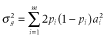, where p_i is the allele frequency at the i^th QTL. The heritabilities of the trait (h²) were set to 0.1, 0.3 and 0.5. To obtain phenotypic values, an environmental effect was added to the true breeding value, which was sampled from a normal distribution as follows: .

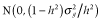After G0, the subsequent 10 generations (i.e. G1 to G10) were generated. In G1 to G10, 30 sires and 30 dams were selected. Each sire was randomly mated to one dam with 10 offspring per mating pair. All sires and dams had five sons and five daughters.

Selection scenarios

Parents from G1 to G5 were randomly selected, whereas those from G6 to G10 were selected on the basis of EBVs. In the selection based on GEBVs, we defined four scenarios regarding the choices of designs for reference populations. In scenario 1, the reference population comprised 3000 animals from G1 to G10. In scenarios 2 to 4, the reference population size was 1500, representing a situation in which the reference population size is limited. In scenarios 2 and 3, the reference populations consisted of all animals in G6 to G10 and G2 to G6, respectively. In scenario 4, the reference population consisted of the half of the animals randomly selected from G1 to G10. The numbers of animals in reference populations are shown in Table 1. The present study assumed that selection candidates had phenotypes before selection. Thus, the reference population included all selection candidates in G6 to G10 for scenarios 1 and 2, only 300 animals in G6 for scenario 3, and half of the selection candidates in G6 to G10 for scenario 4.

We focused on the accuracies of GEBV, additive genetic variances, genetic gains, and inbreeding coefficients at the start (G6) and end (G10) of genomic selection in order to investigate the performance of long-term genomic selection. The accuracies of the GEBVs for selection candidates were calculated from the correlations between GEBVs and true breeding values. The genetic gains were calculated as the cumulative increases of the average breeding values in each generation. The inbreeding coefficients were calculated following Meuwissen and Luo (1992).

Estimation of genomic breeding values

Estimated breeding values were calculated using traditional best linear unbiased prediction (BLUP) to compare estimated breeding values and GEBVs. GEBVs were calculated using single-step genomic BLUP (SGBLUP) on the basis of the integration of phenotypes, SNP markers and pedigree information. The SGBLUP model (Aguilar et al. 2010) was as follows:

where y is the vector of phenotypes, 1_n is the vector of n ones, μ is the mean term, u is the vector of individual additive genetic effects, e is the vector of residuals and Z are incident matrices for u related y. Breeding values were assumed to follow a normal distribution: , where is additive genetic variance and H is the matrix that combines pedigree and genomic relationships. The inverse of H has a simple structure (Aguilar et al. 2010; Christensen & Lund 2010):

where A₂₂ is the sub-matrix of A (pedigree relationship matrix) for the genotyped individuals and G is the genomic relationship matrix. Matrix G was obtained from the following:

where W is the incidence matrix for marker effects and p_j is the frequency of the second allele of genotyped individuals at the j^th marker (VanRaden 2008). Division by makes G analogous to A. The elements of W were calculated as follows:

where m_ij is the number of the second allele of the i^th individual at the j^th marker. Subtracting 2p_j from m_ij sets the mean value of the allele effect at each marker to 0.

Variance components were estimated with average information restricted maximum likelihood (Johnson & Thompson 1995), and the model solutions yielded GEBVs.

Accuracy of GEBVs

In G6, the accuracies of GEBVs in all scenarios were higher than those of the EBVs from BLUP for all heritability levels (Table 2). The differences in the accuracies between GEBVs and EBVs were larger with lower heritability. The accuracies in scenario 3 were higher than those in scenarios 2 and 4 because of the large reference population size. Although the reference population sizes in G6 were 300 and 900 in scenarios 2 and 4, respectively, the accuracies in scenario 4 were lower than those in scenario 2. In G10, the accuracies in scenario 2 were almost equal to those in scenario 1 and higher than those in scenarios 3 and 4 even though the reference populations were the same size. The accuracies in scenario 3 were the lowest among all scenarios in SGBLUP and lower than those in BLUP with heritabilities of 0.1 and 0.3.

Figure 1 shows the accuracies of GEBVs and EBVs from G6 to G10 when heritability was 0.3. In BLUP, the accuracy of EBVs decreased gradually and became almost constant after G8. The accuracies of GEBVs in all scenarios continued to decrease until G10. The accuracy in scenario 3 decreased sharply in G7, and the accuracy was lower than that in BLUP thereafter.

Additive genetic variance

The additive genetic variances in G0 were set to 0.1, 0.3 or 0.5; these values decreased to 0.097, 0.273, and 0.434 in G6, respectively (Table 3). In G10, the reductions in additive genetic variances were larger with higher heritabilities in all scenarios. In particular, these reductions were large in scenarios 1 and 2 because of the high accuracies of GEBVs. The magnitude of reduction in scenario 4 was smallest.

Genetic gain

In G6, the genetic gains in all scenarios were proportional to the accuracies of GEBVs (Table 4). In G10, the genetic gains in scenarios 1 and 2 were large for all heritability levels and about 30% larger than that in BLUP with heritability of 0.1. Among all scenarios in SGBLUP, the genetic gain in scenario 4 was smallest with heritability of 0.1 and largest with heritability of 0.5.

Inbreeding coefficient

In G10, the inbreeding coefficients were highest in BLUP and lowest in scenario 1 for all heritability levels (Table 5). The inbreeding coefficients in all scenarios increased with decreasing heritability. The magnitudes of these increases were large in BLUP and scenario 3. In scenario 4, the inbreeding coefficient was similar to that in BLUP with heritability of 0.5 and lower than that in scenario 3 with heritability of 0.1 or 0.3.

Effect of the extent of LD between QTL on response to selection

In the present study, the total additive genetic variance was calculated as the sum of variances across all QTL. This calculation requires assumption that all QTL are at complete linkage equilibrium. If LD between QTL exists, the additive genetic variance may be underestimated and this underestimated variance may affect the selection response. Here, we investigated the effect of LD between QTL on responses to selection by varying the number of QTL (N_q). The extent of LD was derived from the mean r² value which was the pooled square of the correlation between adjacent QTL. The N_q was varied from 150 to 30. The r² value with N_q of 150 was 0.06 whereas that with N_q of 30 was 0.02. The responses to selection are shown in Table 6. There were no associations between the LD of QTL (or N_q) and the responses to selection.

Accuracy of GEBV

In both BLUP and genomic selection, accuracies were low with small additive genetic variances or low heritabilities. In all scenarios, additive genetic variances decreased with passing generations as described below, reducing accuracy. In particular, in the early selection cycle, the reduction of accuracy was large in scenario 3; this is because the reduction of additive genetic variance was large and there was no marker information for animals after the first selection.

The accuracy of GEBVs is deterministically predicted as follows (Daetwyler et al. 2008):

where N is the number of individuals in the reference population and M_e is the number of independent chromosome segments within the population; this means the number of markers required to tag all potential QTL. M_e can be approximated as 2N_eL, where N_e is the effective population size and L is chromosome length (Hayes et al. 2009b). This formula indicates the accuracy of GEBV increases with a larger reference population size. In G6, the accuracies of GEBVs were highest in scenario 1, because the reference population was largest. However, the accuracies were higher in scenario 2 than scenario 4 for all heritability levels despite the large population sizes in scenario 4; this is due to the degrees of the relationships among genotyped individuals. The above formula assumes there are no relationships between candidates for selection and the reference population or within the reference population. In reality, the accuracy of GEBV is affected by these relationships (Habier et al. 2010; Pszczola et al. 2012). Clark et al. (2012) demonstrate that candidates more closely related to the reference population have more accurate GEBVs. Thus, the present results indicate the addition of distantly related individuals to the reference population might contribute little to improving the accuracy of GEBVs as observed in scenario 4. Therefore, the relatedness between the reference population and candidates should be considered in order to obtain high accuracy.

Additive genetic variance

Assuming an infinite number of unlinked loci with an additive genetic effect, direct selection leads to the reduction of additive genetic variance. When selection is performed for several generations, additive genetic variance reaches an equilibrium value between additive genetic variance before selection and Mendelian sampling variance (Bulmer 1971). Van Grevenhof et al. (2012) deterministically predicted this equilibrium value after long-term genomic selection according to the following formula:

where k is the proportional reduction in the variance of the selection criterion as a result of the selection of the parents, and and are the additive genetic variance and accuracy of GEBV before selection, respectively. According to this formula, in G10, the additive genetic variances in scenarios 1 and 2 were small because of the high accuracies of GEBVs. However, when heritability was 0.5, the additive genetic variance was larger in scenario 4 than scenario 3 despite higher accuracy. The prediction formula assumes all candidates for selection have marker information. The accuracies in scenarios 3 and 4 might not be calculable using this formula, because there were candidates without marker information.

Genetic gain

For long-term selection, it is most important to improve genetic gain at the end of selection. In G10, there were no differences in the genetic gains between scenarios 1 and 2 for all heritability levels. When heritability was 0.5, the genetic gain was highest in scenario 4. In scenario 1, the additive genetic variance decreased quickly because of the high accuracy in early selection cycles. This reduction led to the losses of genetic gains in later selection cycles. These results indicate long-term genetic gain can be improved by creating an appropriate design for the reference population that considers the degree of heritability, even if the reference population size is limited.

The present study investigated the response of genomic selection over five generations (i.e. G6 to G10). The accuracies of GEBVs and the additive genetic variances decreased with passing generations. Therefore, the advantages of genetic gains from the four scenarios will change over the course of more than five generations. When considering such long-term selection, the genetic gains from genomic selection can be predicted on the basis of the present results about patterns of accuracies and additive genetic variances.

Inbreeding coefficient

Several simulation studies show that inbreeding coefficients increase with decreasing heritabilities in long-term BLUP selection (Belonsky & Kennedy 1988; Kuhlers & Kennedy 1992; Satoh 2004). In the present study, the same results were obtained when both BLUP and genomic selection were applied. However, genomic selection led to a smaller increase in the inbreeding coefficient with lower heritability. In particular, the results of scenarios 2 to 4 indicate it is desirable to add individuals in later generations of long-term selection to the reference population.

The inbreeding coefficients used in the present study were calculated from pedigree information and describe the probability that two alleles at a randomly chosen locus were identical by descent (IBD). Although this pedigree measure of inbreeding is supposed to capture the genome-wide increase in homozygosity, it may not be the most relevant measure if genetic variance due to a few QTL or selection changes in allele frequencies at specific genome positions (Bastiaansen et al. 2012). Accordingly, Sonesson et al. (2012) recommend genome-based inbreeding coefficients be calculated from the probability of IBD based on both pedigree and marker information when applying genomic selection.

Selection strategy

The present study proposed four scenarios for choices of reference populations with five generations of genomic selection and assumed all candidates for selection were phenotyped before selection. Of course, there are several other options for constructing reference populations. Bastiaansen et al. (2012) compared two designs for reference populations consisting of one and five generations, respectively. Jannink (2010) proposes two phenotyping schemes in which all selection candidates are phenotyped before or after selection. The results of these studies and the present study will aid the selection of an optimum design for reference populations.