1 INTRODUCTION

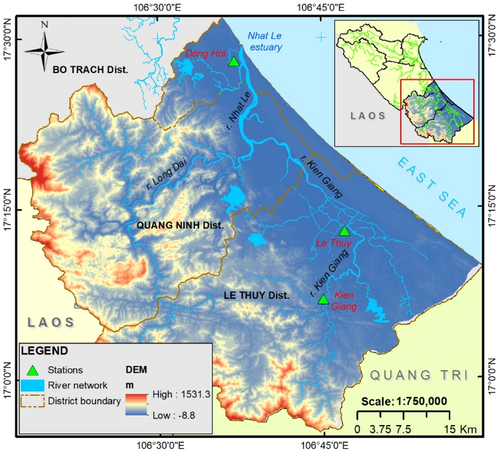
The Kien Giang River, a tributary of the Nhat Le River, flows through Le Thuy and Quang Ninh districts in Quang Binh Province with a length of 69 km (Figure 1) (Ly et al., 2013). It originates from the Annamite Range (Truong Son Range), with various streams contributing to its waters. Due to the rugged terrain of the upper Kien Giang river basin, rainwater from the Annamite Range flows vigorously towards its lower reaches in the rainy seasons (autumns), causing floods across the basin. Diverging from the southeast trajectory characteristic of most Vietnamese rivers, the Kien Giang River flows northeast and creates a narrow delta in Le Thuy and Quang Ninh districts. The Kien Giang River meets the Long Dai River at Tran Xa junction in Quang Ninh district, together creating the Nhat Le River.

Accurate water level prediction is critical for early flood warning and flood disaster mitigation. In general, two main approaches are adopted to predict the water level. The first approach heavily relies on physically-based models, such as the MIKE HYDRO River, HEC-HMS, SOBEK, EFDC, and so forth. Although these models provide high accuracy in water level prediction, they require a variety of datasets, including topographic, meteorological, and hydrological data, and a long time for model simulation. Therefore, physically-based models are unsuitable for short-term and real time predictions. Moreover, physically-based modeling often demands in-depth knowledge and expertise in hydrological domains (Bao et al., 2017).

An alternative approach is to utilize data-driven models to collect and analyze statistical relationships between input and output data. This strategy can remove the previously outlined limitations of physically-based models. Notably, Quang et al. (2022) used data-based regression models to forecast the water level in the Kien Giang River. Chau (2006) and Castillo et al. (2018) used Artificial Neural Network (ANN) to predict the water level. Recently, Machine Learning (ML) has been increasingly used alone or in combination with other process-based models. The advantage of ML is that various techniques can be applied depending on the user's application purpose. Given that each technique has also shown good performance, ML can complement the limitations of physical processes based on complex theories and mathematical equations. Since 1990s, water level prediction has been conducted using various neural network modeling techniques to improve the accuracy (Booker & Woods, 2014; Jothiprakash & Magar, 2012; Konstantine et al., 2004; Shamseldin & O'Connor, 1999; Tiantian et al., 2016; Young & Liu, 2015). ML can be classified into supervised learning and unsupervised learning, depending on the presence or absence of the dependent variables (Jungho et al., 2019). Representative supervised learning methods for classification and regression include Decision Tree (DT) (Quinlan, 1986), Random Forest (RF) (Breiman, 2001), and Support Vector Machine (SVM) (Vapnik, 1999). K-means for clustering (MacQueen, 1967) and self-organizing maps (Kohonen, 1982) are representative unsupervised learning techniques.

In recent years, Deep Learning (DL) techniques such as Convolutional Neural Network (CNN) and Recurrent Neural Network (RNN) have been integrated into water monitoring systems. Among these, Long Short-Term Memory (LSTM)—a type of RNN has been widely applied in performing prediction tasks, particularly in the time series modeling. Sahoo et al. (2019) investigated the use of LSTM-RNN for low-flow hydrological time series prediction at the Basantapur station in the Mahanadi River, India. The study showed that LSTM-RNN outperformed both RNN and naive methods. Le and Lee (2019) employed LSTM to forecast the discharge at the Hoa Binh station in the Da River, Vietnam where the flow rate and rainfall observations from several meteo-hydrological stations before the construction of the Hoa Binh reservoir were used. The results revealed that LSTM achieved over 86% of accuracy for 1-, 2-, and 3-day forecasts. Sankaranarayanan et al. (2020) proposed the Deep Neural Network for flood occurrence prediction using temperature and rainfall intensity data. Tao et al. (2020) adopted Multilayer Perceptron (MLP) and RNN to develop two models for forecasting the water level with 2- and 6-h lead time.

This paper aims to develop DL models using DL network architectures of GRU, LSTM, and Bi-LSTM to predict the water level at the Le Thuy station in the Kien Giang River.

2 METHODOLOGY AND STUDY AREA

2.1 DL models

DL model, or neural network (NN) model, is a branch of ML models inspired by the operations of biological systems such as biological brains. It attempts to learn a detailed representation of the output by progressively feeding the inputs through one or more than one hidden layers. For time series analysis tasks such as water level prediction, RNN and its variants are widely used because of its unique ability to accept inputs as a sequence of data and allow the information learned in prior time steps to inform the prediction in subsequent time steps.

2.1.1 Recurrent neural network (RNN)

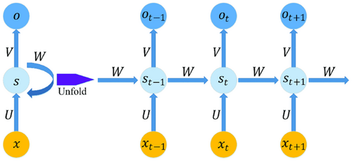
Robinson and Fallside (1987) first introduced a model that, instead of using the entire sequence of inputs X, sequentially uses the input at time step t to predict the output (Figure 2). The cell state s_t is updated with both the previous time step cell state and the input, and then the output o_t is computed using the cell state s_t. Formulas for the hidden state s_t and output o_t are shown below:

where U, V, W are the weights for the input, recurrent connections and cell state, respectively; s_t−1, s_t are cell state at time step t − 1 and t; are the biased terms; and f, g are activation functions.

2.1.2 Long-short term memory (LSTM)

The problem with RNN models arises when they are trained on very long sequences of data, as the propagated error signals either explode or vanish (Hochreiter & Schmidhuber, 1997). This is a typical problem in ML literature, as either the model cannot converge with its weights oscillating wildly in the case of exploding gradients, or it eventually stops learning as the gradients approach 0 in the case of vanishing gradients. As a result, Hochreiter and Schmidhuber (1997) proposed a new model architecture, in which the input would go through a memory cell. The memory cell contains two multiplicative “input” and “output” gates to control the flow of information going in and out of the cell. In a subsequent paper, Gers et al. (2000) extended the model to include a third “forget gate” to gradually reset the memory cell (Figure 3). 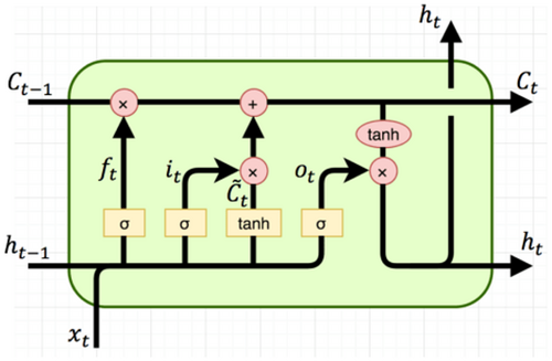Formulas for the different gates f_t, i_t, o_t; the temporary memory cell ; the memory cell c_t; and the output o_t at time step t are shown below:

where W_q and U_q are weights for the inputs and the recurrent connections, and the subscript q can either be the input gate I, the output gate o, the forget gate, f, or the memory cell c; are biased terms; and , are activation functions.

2.1.3 Bidirectional long-short term memory (Bi-LSTM)

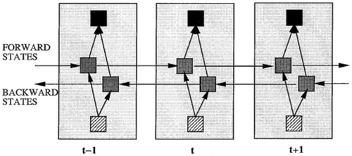
Another problem with RNN models, as well as with LSTM, is its inability to analyze data backwards (from the future to the past). In applications such as text or music, humans need to consider the entire sentence or a musical interval to understand its context. To address this problem, Schuster and Paliwal (1997) first proposed a bidirectional RNN (BRNN) model, which consists of two separate RNN models that consecutively process the inputs forward in time and backward in time (Figure 4). Alex and Jürgen (2005) extended this concept by replacing the RNN components with LSTM to develop Bidirectional LSTM (Bi-LSTM).

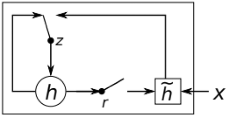
2.1.4 Gated recurrent unit (GRU)

As an alternative to LSTM, Cho et al. (2014) proposed a simpler model architecture only consisting of “reset” and “update” gates. In a GRU block, the update gate z decides whether to use the current or previous time step unit, and the reset gate decides whether to ignore the previous time step unit when calculating the current time step unit (Figure 5). Formulas for the different gates r_t, z_t; the proposed unit _t, and the new unit _t at time step t are shown below:

where W_q and U_q are weights for the inputs and the recurrent connections, and the subscript q can either be the reset gate r, the update gate z, or the unit h; are biased terms; and are activation functions.

2.2 Metrics

For water level prediction, studies have proposed R² (Coefficient of determination), RMSE (Root Mean Squared Error) and MAE (Mean Absolute Error) metrics to evaluate the performance of DL models (Atashi, 2022; Ryan et al., 2021).

where and are the observed and predicted water level; and are the mean of observed and predicted water level. The value of ranges from 0 to 1; where 1 indicates predicted values are close to true values. MAE and RMSE are two metrics indicating the model's errors with the optimal value being close to 0.

We also proposed two additional metrics, that is, Max Error Value (MEV) and Max Error Time (MET), as it is crucial for our models to correctly predict the flood peak as well as its timing. The flood in the Kien Giang River at 6:00 on October 19, 2020 recorded a historic water level of 4.88 m. We aimed to not only predict the peak value as close as possible, but also within a 6-h span before and after it. The metrics formulas are expressed as follows:

where argmax() is the function that returns the row id of a series.

MEV and MET are two specific metrics in our paper indicating the model's errors regarding the flood peak with the optimal value being close to 0.

2.3 Study area and data collection

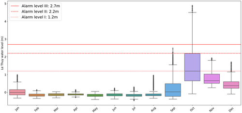
The Nhat Le river basin mainly consists of three rivers, that is, Kien Giang, Long Dai, and Nhat Le, with a total area of 2612 km² (Figure 1) (Ly et al., 2013). There are three meteo-hydrological stations namely Kien Giang, Le Thuy, and Dong Hoi in the basin that measure rainfall and water level over a long period. In this study, the hourly water level data for four major flood years (2010, 2012, 2016, 2020) and the available hourly rainfall data for 2 years (2016 and 2020) of those three stations are collected. The Box and Whisker plot in Figure 6 shows that significant water level rise on the Kien Giang River often occurs from September to December, corresponding to the flood season in the study area (Ly et al., 2013).

Due to the dispersion of the collected data, we processed each year separately before concatenating them into the final data set. After that, the final data set was split into the training set and validation set with a ratio of 80%–20% for model development and evaluation purposes. It is also worth noting that since the hourly rainfall data for 2010 and 2012 is not available, we decided to exclude the hourly water level in those 2 years when both water level and rainfall data are used in the data set. Concretely, the data set using only water level data has 21,268 and 5318 data points for training and testing, respectively; while the data set using both water level and rainfall data has 14,052 and 3514 data points for training and testing, respectively.

3 DATA INPUTS AND MODEL DESIGN

Three RNN-based DL models were employed to develop the data-driven model to predict the water level at the Le Thuy station. Partial Autocorrelation function (PACF) of the water level was analyzed to select the optimal data inputs for the models. Several time leads were selected to evaluate the forecast capability of the models. Five metrics, that is, R², MAE, RMSE, MEV, and MET were used to evaluate the performance of the models. The models were developed in Python 3.7 using the DL framework Keras Pytorch.

3.1 Selection of optimal data inputs

3.1.1 Selection of the number of time lags and time leads

For water level prediction, data-driven models leverage historical rainfall, water level, and so forth to predict future data. Therefore, the selection of the number of time lags and time leads used for data inputs can have a significant effect on the forecast capability of the models.

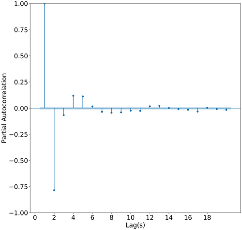
In time series analysis, PACF is a reliable tool that can be used to identify the order of an autoregressive model (Box George et al., 2008). It calculates the partial correlation of a stationary time series with its own lagged values while regressing the values of the time series at all shorter lags. The PACF plot for the water level at the Le Thuy station in Figure 7 shows that 9 is the last value after which all the time lags are within the confidence interval. Due to the number of scenarios and model architectures, 3-time lags (1, 4, and 9 h) were selected to represent low, medium, and high number of time lags for our inputs.

At the same time, the number of time leads is also hard to select. A low number of time leads indicates that the outputs correlate more closely with the inputs, therefore making it easier for a ML model to predict. However, it is more desirable for the model to predict further into the future during flood events, at the cost of less input-output correlation. As a result, 4 time leads (1, 3, 6, and 12 h) were selected to validate the forecast capability of each model.

3.1.2 Scenarios

Once the number of time lags and time leads were selected, we proceeded to set up combination of inputs and output used by the models. In this study, three scenarios were established for our experiments (Table 1):

• 1.

  SC1: The hourly water level at three stations from time lags t – m to t;

• 2.

  SC2: The hourly water level and rainfall at three stations from time lags t – m to t;

• 3.

  SC3: The hourly water level and rainfall at three stations from time lags t – m to t, and the total hourly rainfall forecast at three stations from time leads t to t + n.

where m and n are the number of time lags (1, 4, and 9 h) and time leads (1, 3, 6, and 12 h).

Table 1. Scenarios of input–output combinations for model development and validation.

Scenario	Inputs			Output
	Hourly water level at 3 stations	Hourly rainfall at 3 stations	Total rainfall forecast at 3 stations
SC1	Ht, Ht–1, …, Ht–m	-	-	Ht+n
SC2	Ht, Ht–1, …, Ht–m	Rt, Rt−1, …, Rt−m	-	Ht+n
SC3	Ht, Ht–1, …, Ht–m	Rt, Rt−1, …, Rt−m	Rt + Rt+1 + … + Rt+n	Ht+n

The third input, that is, the total rainfall forecast, is considered as a potential candidate in SC3 due to two reasons. First, the difference between water level at the time step t and t + n depends on the amount of rainfall in-between that time, and this information is not a part of the historical water level. Second, rainfall forecast incorporates information from different sets of inputs that our data set cannot capture, which can assist the models in learning a better representation of the outputs. Since our data set does not contain the historical total rainfall forecast, we simulated the input by calculating the sum of rainfall from time leads t to t + n.

3.1.3 Configuration of the models

When setting up the configurations for training a DL model, some parameters are needed to be considered, as shown in Table 2. The first parameter is the number of layers. A DL model with a high number of layers can learn much more complex representations of the input data than one with fewer layers. In this paper, we have experimented with three models with one, two, and three LSTM layers, respectively (Figure 8). The results demonstrated that the number of layers has a slightly negative correlation with our metrics. As a result, we decided to use one layer as the standard for all three models to shorten the training time.

Table 2. Final input–output combinations for model development and validation.

Parameter	Value
Number of layer(s)	1
Number of hidden unit(s)	150
Optimizer	Adam
Loss function	MSE
Batch size	256
Learning rate	1e−3

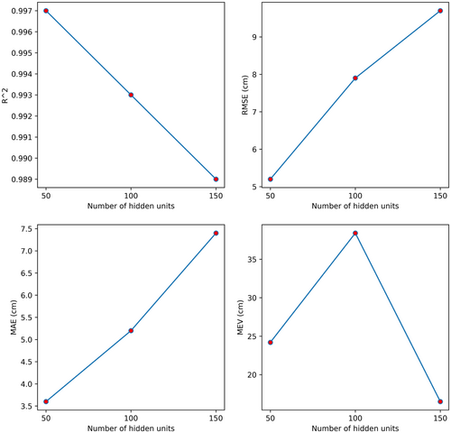
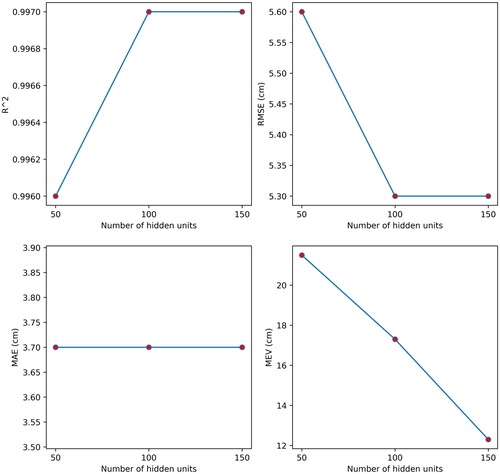
The number of hidden units in each layer is another key parameter in DL models. A model with fewer hidden units tends to generalize better but predict less accurately, while a model with more hidden units can predict better but is more prone to overfit. We have experimented with three LSTM models with 50, 100, and 150 hidden units (Figure 9). The results showed that although our first three metrics were not improved significantly, the increase in the number of hidden units improved the model's ability to predict the flood peak with a MEV decreasing from 0.215 to 0.123. Therefore, we used 150 hidden units as the standard for all three models.

Adam optimizer was selected as it is one of the standard optimizers for different DL tasks. Additionally, the Mean Squared Error (MSE) was used as the loss function because it is closely related to the RMSE and MAE metrics. The number of batch size plays a less significant role in model development. A high batch size will help the model generalize better as the weights and losses are updated on a bigger sample size. However, in other DL tasks such as object detection, due to the size of each sample, it is more ideal to compromise model generalization for shorter training time. Finally, the standard learning rate was set at 1e−3 as we observed smooth training and validation loss curves during model training. We also didn't apply any fixed number of iterations for our models, as we set up an early stopping callback in case of no improvements in the models for three iterations.

4 RESULTS AND DISCUSSIONS

In this study, a total of 108 different models based on different scenario inputs, time lags, and time leads has been developed. The results at the scenario level are aggregated in Table 3. For example, the R² of Scenario SC1 with a time lead of 1 h is the average value of R² of nine models (three of each LSTM, GRU, and Bi-LSTM models built with three different time lags). Two general trends can be observed from the obtained results: (i) given the same model and number of time lags, the metrics worsen as the predictions extend further into the future with more time leads, and (ii) given the same model and the number of time leads, the metrics also worsen as we use more time lags (Table 4). Of all scenarios and time leads, the models using Scenario SC2 and predicting water level with 1-h time lead provided the best average metric.

Figure 10 shows a clear separation between the observed and predicted water level at the Le Thuy station as more time lags were added into the three models. All three models can form a good correlation between observed and predicted data when the water level did not exceed Alarm level III, that is, 2.7 m. However, due to the unique nature of the historical flood on October 19, 2020, the models diverged in two different directions as the observed water level increased above 3.2 m: GRU and Bi-LSTM models overestimated the water level, while LSTM model slightly underestimated it. This difference became more apparent as the number of time lags increased, for example, when using time steps t − 9 to t, the Bi-LSTM model predicted even higher than actual values, while the LSTM model predicted even lower than actual values. However, it can be observed that some of GRU's predictions started to converge back to the 1:1 line when adding more time lags.

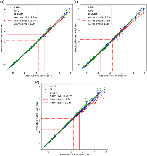
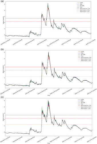
Figure 11 compares the observed and predicted water levels of three models based on tested data. To predict the peak of the flood event, the LSTM model using time lags t − 1 to t performed the best out of nine models with only a 3.6 cm difference, and it also predicted the flood peak 1 h earlier. Interestingly, three other models (LSTM using time lags t − 9 to t, Bi-LSTM using time lags t − 1 to t, and Bi-LSTM using time lags t − 9 to t) correctly predicted the time of the flood peak but with higher difference in water level values.

5 CONCLUSIONS

In this paper, three DL models, namely LSTM, GRU, and Bi-LSTM, have been developed to predict the hourly water level at the Le Thuy station in the Kien Giang River. The hourly rainfall and water level data set at three meteo-hydrological stations in four major flood years have been collected for model development and validation.

The findings highlight that the input scenario using water level and rainfall from time step [t − 1, t] of three stations to predict the water level at the Le Thuy station with 1-h time lead, provides the best results both in term of peak flood events and overall water level trends. Statistical metrics, including , RMSE, MAE, MEV, and MET, demonstrate the application potential of DP models in water level prediction. Among the evaluated models, the LSTM model outperforms GRU and Bi-LSTM models.

In future studies, authors will consider gathering more data and supplementary inputs such as stream flows, runoffs from sub-catchments, tidal level, and so forth. Meanwhile, different architectures of the three models used in this study and other types of DL models should be explored to improve the accuracy of water level predication.

ETHICS STATEMENT

None declared.