Orientational anisotropy of bead-spring star chains during creep process
Abstract
The bead-spring model for star chains (Rouse–Ham model) is a fundamental model for the polymer dynamics. Despite the importance of this model, its dynamics under the stress-controlled condition was not analyzed so far. For completeness of the model, the equation of motion of the Rouse–Ham chain was solved to derive an analytical expression of the orientation function S(n,t) for the stress-controlled creep process. This expression indicated that the segments near the free end of the star arm exhibit overshoot of their orientational anisotropy to compensate for the slow growth of the anisotropy near the branching point and that the distribution of the anisotropy along the arm contour becomes more heterogeneous with increasing arm number f. This correlation/interplay of the segments at different locations along the arm, not seen under the strain-controlled condition, is a natural consequence of the constant-stress requirement during the creep process. The corresponding interplay was noted also for respective Rouse–Ham eigenmodes. © 2006 Wiley Periodicals, Inc. J Polym Sci Part B: Polym Phys 44: 3501–3517, 2006
INTRODUCTION
The bead-spring model of the flexible chains has been widely utilized as the model of non-entangled flexible chains as well as the starting framework of the tube model for entangled chains.1-3 Under the strain-controlled conditions such as the step-strain and constant-rate flow, the dynamics of the bead-spring chains has been fully analyzed in literature and the fundamental linear viscoelastic properties such as the relaxation modulus G(t) and complex modulus G*(ω) have been formulated with no ambiguity.1-3 Nevertheless, no analysis was made for the chain dynamics under the stress-controlled condition and no analytic expression of the transient creep properties (such as the creep compliance J(t)) was reported in literature.
This lack of the analysis of the dynamics under the stress-controlled condition was quite surprising when we thought about the fundamental importance of the bead-spring model. Thus, for completeness of the model, we recently made this analysis for linear chains obeying the Rouse dynamics.4-8 The analysis indicated that the Rouse eigenmodes of different orders, being independent under the strain-controlled condition, have correlated amplitudes during the stress-controlled creep process.4, 6 The correlation also emerges for long and short chain components in blends during the creep process.7 These features naturally result from the constant-stress requirement during this process and the general stress-optical rule. The analysis also revealed that the Rouse chain exhibits the affine deformation on sudden imposition of a stress.5, 8 Furthermore, the analysis gave an analytic expression of J(t) as a byproduct.4, 7, 8
In this study, we extend our analysis to the dynamics of the bead-spring star chain (Rouse–Ham chain9, 10) during the linear viscoelastic creep process. Specifically, we start from the equation of motion of this chain to calculate the orientation function that specifies the magnitude of orientational anisotropy of respective segments in the star arm. The results, including those for the linear Rouse chain as a special case, are discussed in relation to the correlation/interplay of segments along the star arm and of the Rouse–Ham eigenmodes.
RESULTS
The Model and Outline of Calculation
We consider a monodisperse system of symmetric f-arm star chains obeying the Rouse–Ham dynamics9, 10 (Zimm–Kilb dynamics11 in the free-draining limit). Each arm is composed of N (≫1) segments having the friction coefficient ζ. Neighboring segments are connected with the Gaussian spring of equilibrium length a and spring constant κ = 3kBT/a2 (kB = Boltzmann constant, T = absolute temperature); cf. Figure 1. For each arm, the segment index n runs from 0 to N, where n = 0 and N specify the branching point and free end of the arm, respectively.
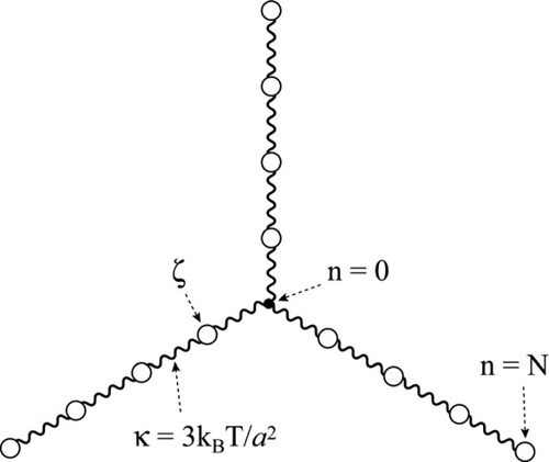
Schematic illustration of a three-arm bead-spring star chain (Rouse–Ham star chain).
 (1)
(1)Here, r (n, t) is the ξ component (ξ = x, y) of the spatial position r[α] (n, t) of the n-th segment in α-th arm at time t, ∂r[α] / ∂n denotes the bond vector for this segment, and 〈 … 〉 represents an ensemble average. S[α] (n, t) is the orientation function of the α-th arm, and S(n,t) is defined as the average over all f arms.
 (2)
(2)Here, ν is the number density of the chains in the system. The time evolution of S(n,t) during the creep process is determined by the Rouse–Ham dynamics under the constraint that σ(t) is kept constant (=σ0). This constraint results in the interplay/correlation of the Rouse–Ham eigenmodes, as discussed later in more details.
Equation of Motion
 (3)
(3) (4)
(4) (5)
(5)Here,
 represents the strain rate at time t (uniform in the system), and the x- and y-directions are chosen to be the velocity and velocity gradient directions, respectively.
Boundary Condition and Eigenmode Expansion
 (6)
(6) (7)
(7) (8)
(8) (9)
(9) (t; p) with η = o and e represent the amplitude vectors of the p-th order odd and even eigenmodes for α-th arm at time t. The amplitudes for the f arms are not totally independent but are correlated through the boundary conditions, eqs 7 and 8. The even modes appearing in eq 9 automatically satisfy eq 8 but their amplitudes B
 are subjected to a constraint due to eq 7,11
 (10)
(10) are subjected to a constraint due to eq 8,11
 (11)
(11)Thus, among the p-th order eigenmodes for the f arms, only one even mode and f−1 odd modes behave as the independent eigenmodes.
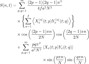 (12)
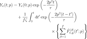
(12)Here, X (t; p) and Y
 (t; p) represent the x and y components of B
 (t; p), respectively, and Xe (t; p) and Ye (t; p) denote those of Be (t; p). (In eq 12, the cross terms between the odd and even modes vanish because of eqs 10 and 11.) Solving the equation of motion (eq 3), we can calculate the averages 〈XY〉 appearing in eq 12 and obtain an explicit expression of S(n,t).
Eigenmode Analysis
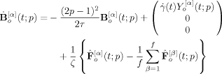
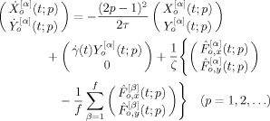
 (t; p) and Be (t; p). Details of this derivation are described in Appendix A, and the equations for the x and y components of these vectors relevant to the calculation of S(n,t) (eq 12) are summarized as
 (13)
(13) (14)
(14) (15)
(15) (t; p) and F̂
 (t; p) indicate the ξ components (ξ = x, y) of the p-th order sine- and cosine-Fourier components of the Brownian force acting on β-th arm,
 (16)
(16) (17)
(17) (t; p) (η = o, e and ξ = x, y) is given by
 (18)
(18)Note that eqs 13 and 14 are written for each arm but include the Fourier components of the Brownian forces acting on all arms. This feature, representing the coupled motion of the arms, results from the boundary conditions, eqs 10 and 11.
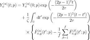
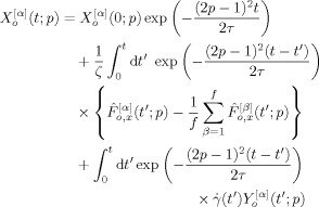
 (t; p) and X
 (t; p) for p-th odd mode:
 (19)
(19) (20)
(20) (t; p) Y
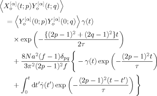
 (t; q)〉 term included in the orientation function (eq 12) can be straightforwardly calculated. Although eqs 19 and 20 show that this term is contributed from several types of averages such as 〈X
 (0; p) Y
 (0; q)〉 and 〈X
 (0; p) F̂
 (t′; q)〉, most of these averages vanish: For example, 〈X
 (0; p) Y
 (0; q)〉 = 0 because the chains are at equilibrium at t = 0 (just before application of the stress) to have an isotropic conformation with no correlation between X
 (0; p) and Y
 (0; q), and 〈X
 (0; p) F̂
 (t′; q)〉 = 0 because the chain conformation at t = 0 is not correlated with the Brownian force at time t′ > 0. From a careful inspection of eqs 19 and 20, we note that the 〈X
 (t; p) Y
 (t; q)〉 term has nonzero contributions only from two types of averages, 〈F̂
 (t′; p) F̂
 (t″; q)〉 and 〈Y
 (0; p) Y
 (0; q)〉, and is written, after some calculation, as
 (23)
(23) (t′; p) F̂
 (t″; q)〉 and 〈Ye (0; p) Ye (0; q)〉, and written as
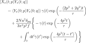 (24)
(24)In derivation of eqs 23 and 24, we have utilized eqs 15 and 18 to specify 〈F̂ (t′; p) F̂
 (t″; q)〉 (with η = o, e) and τ, respectively.
 (0; p) Y
 (0; q)〉 and 〈Ye (0; p) Ye (0; q)〉, can be calculated from the equilibrium distribution function of the eigenmode amplitudes, as explained in Appendix B. The results are summarized as
 (25)
(25) (26)
(26) (27)
(27)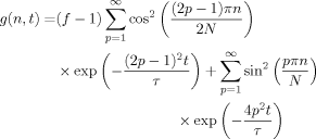 (28)
(28)Note that this S(n,t) is contributed from no cross-average between the odd and even eigenmodes.
Calculation of S(n,t)
 , eqs 27 and 28 give
 (29)
(29) (30)
(30) , eqs 27 and 28 give
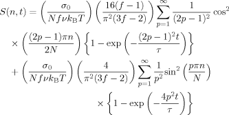 (31)
(31) by a ratio of the steady state stress σ0 to the zero-shear viscosity η0 and further utilized the expression of η0:12
 (32)
(32) is not externally given but determined by the chains themselves under the requirement of constant stress σ0. Equations 2, 27, and 28 give the equation that determines
  :
:
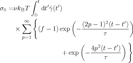 (33)
(33)As can be noted from eq 30, eq 33 is equivalent to the linear viscoelastic constitutive equation,
 with
with  for t′ < 0 (where the stress has not been applied).
 (34)
(34) (35)
(35) (36)
(36) (37)
(37) (38)
(38) (39)
(39)| p | φp/π | ||
|---|---|---|---|
| f = 2 | f = 3 | f = 8 | |
| 1 | 0.7151 | 0.7821 | 0.8776 |
| 2 | 1.2295 | 1.1819 | 1.1094 |
| 3 | 1.7354 | 1.7946 | 1.8816 |
| 4 | 2.2387 | 2.1883 | 2.1121 |
| 5 | 2.7408 | 2.7980 | 2.8828 |
 (with J(t) being given by eqs 34–36) in eq 27, we can find an expression of S(n,t) with the Laplace transformation method described in Appendix D. The results are summarized as
 (40)
(40) (41)
(41) (42)
(42)For f = 2, all above results reduce to those for the linear Rouse chain obtained previously.4, 8 Namely, for f = 2, eq 37 reduces to the previously derived eigenvalue equation for the linear chain, tan θq = θq with θq = 2φq. Correspondingly, the expression of JR(t) (eqs 35 and 36) reduces to the previous expression. The expression of S(n,t), eqs 40–42, were obtained after analytical summation of the eigenmodes of g(n,t) in the Laplace space (as described in Appendix D) and thus superficially different from the previous expression formulated before this summation (eqs 13 and 27 in ref.4). However, no real difference exists between the present and previous expressions of S(n,t), as explained later for the anisotropies of the eigenmode amplitudes.
DISCUSSION
Anisotropy Distribution along the Arm Contour
For the Rouse–Ham star chains with various arm numbers f, Figure 2 shows the normalized orientation function during the creep process, S° (n, t) = {NfνkBT/σ0} S(n, t) (eq 40). This S° (n, t) is plotted against the normalized segment coordinate, n/N, at several reduced times, t/λ1 = 0.01, 0.1, 0.3, 1, and ∞, with λ1 being the longest retardation time (eq 36). For comparison, Figure 3 shows S° (n, t) after start-up of constant-rate flow (eq 31); the plots are shown at t/τ = 0.01, 0.1, 0.3, 1, and ∞, with τ being the longest relaxation time (eq 15). In both figures, the plots for f = 2 indicate the orientation function of the linear Rouse chain composed of 2N segments, and n = 0 corresponds to the segment at the chain center.
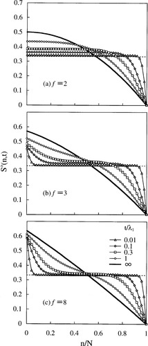
Changes of the normalized orientation function S° (n, t) of Rouse–Ham star chains with various arm numbers f during the creep process.
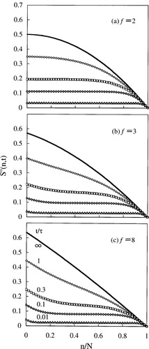
Changes of the normalized orientation function S° (n, t) of Rouse–Ham star chains with various arm numbers f after start-up of constant rate flow.
In Figure 2, the horizontal dotted line indicates the S° value expected for the affine deformation against the stress σ0 (uniform deformation along the arm contour); S°affine = 1/3. For all f values, S° (n, t) during the creep process at short t is only weakly dependent on n and its value in the major part of the range of 0 < n/N < 1 is close to this affine value; see the plots at t/λ1 = 0.01 (triangles). In fact, in the limit of t → 0, eq 40 gives S° (n, t) = S°affine in the entire range of 0 < n/N < 1 irrespective of the arm number f. This affine deformation enables the chain having finite retardation times to instantaneously respond to the applied stress, as fully discussed in the previous papers.5, 8 Note also that thenon-normalized orientation function has an infinitesimal value on the affine deformation, S(n,0) = σ0/3NfνkB T → 0 for N → ∞, which corresponds to an infinitesimal value of the initial compliance, J(0) → 0 for N → ∞.
As seen in Figure 2, the flat, affine profile of S° changes with t in a way that the S° (n, t) value increases and decreases, respectively, for the segments near the branching point (n/N = 0) and the arm end (n/N = 1). Namely, S° (n, t) of the segments near the arm end approaches its steady state (S° (n, ∞) shown with the thick solid curves) after exhibiting the overshoot at short t. This overshoot is a natural consequence of the constant-stress requirement during the creep process: The total orientational anisotropy, being equivalent to the stress (cf. eq 2), is kept constant during this process, but the segments near the branching point cannot quickly attain their steady state anisotropy. (The anisotropy near the branching point grows considerably even at short t but the final growth to the steady state value occurs only slowly in a time scale of t ≥ λ1; cf. Fig. 2.) Thus, the segments near the arm end, which can relax faster than the branching point segment, compensate for the delay in this final growth near the branching point by exhibiting the overshoot at short t. In other words, the overshoot reflects the interplay of the segments along the arm contour under the constant-stress requirement.
After start-up of the constant rate flow, S° (n, t) changes with t quite differently: As seen in Figure 3, S° (n, t) of all segments monotonically increases with t, and the approach to S° (n, ∞) is faster for the segments near the arm end. Thus, qualitatively speaking, the segments along the arm contour can determine their orientational anisotropy more independently under the constant-rate flow than in the creep process (because of the lack of the constant-stress requirement for the former). This difference between the creep and constant-rate flow processes can be noted also for the anisotropy of the eigenmode amplitude explained later.
Qualitatively, the above features are common to the star chains of any arm number f (including the linear chain with f = 2). However, we also note a quantitative difference for the star chains with various f. This difference can be most clearly demonstrated in Figure 4 where the S° (n, t) profiles of the stars with various f during the creep process are directly compared.
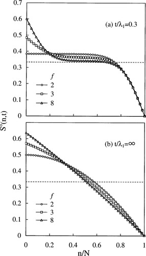
Direct comparison of the normalized orientation function S° (n, t) of Rouse–Ham star chains with various arm numbers f.
 (43)
(43)Of course, this S° (n, ∞) profile coincides with that under the rate-controlled flow given by eq 31 with t → ∞. (This coincidence can be easily noted by applying mathematical formulae,14, 15 Σ p−2 cos px = { 3(x − π)2 − π2} /12 for 0 ≤ x ≤ 2π and Σ
 (2p − 1)−2 cos (2p − 1)x = π (π − |2x|) /8 for −π ≤ x ≤ π, to eq 31.)
As seen in Figure 4(b), the negative gradient of the steady state profile at n/N = 0, [dS° (n, ∞) / d }n / N}]n/N = 0, is enhanced with increasing f > 2 (and approaches −2/3 for f → ∞; cf. eq 43). Thus, the orientational anisotropy in the steady state is more heterogeneously distributed along the arm contour for larger f. This behavior is a natural consequence of the fact that the branching point is subjected to the tensile forces from all arms and thus has a larger, steady state orientation for larger f. Since the total orientation is kept constant during the creep process, the enhancement of the orientation near the branching point reduces the orientation of the segments far from this point, thereby giving the larger heterogeneity for larger f.
The situation is essentially the same in the transient state at t/λ1 = 0.3 [cf. Fig. 4(a)]. The orientation near the branching point is enhanced for larger f, as explained above. Under the constant-stress (constant total orientation) requirement, this enhancement allows S° (n, t) of the middle part of the arm (at around n/N = 0.5) to remain closer to the initial affine profile (S° (n, 0) = 1/3) shown with the horizontal dotted line.
Anisotropy of Eigenmode Amplitudes
 (44)
(44) (45)
(45)For f = 2, this definition reduces to the previous definition4 for the linear Rouse chain (composed of 2N segments).
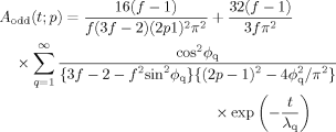
The t dependencies Aodd and Aeven represent the change of the orientational anisotropy of the star chain through the odd and even eigenmodes, the former involving no motion of the branching point while the latter activating the synchronized motion of all arms and being associated with the motion of the branching point. Aodd and Aeven can be determined from a rheo-optical experiment for a series of star chains having the same architecture and differently located optical label and Fourier analysis of the resulting rheo-optical data with respect to the label location.4
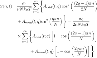 (46)
(46) (47)
(47) (48)
(48) (49)
(49)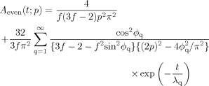 (50)
(50)For f = 2, eqs 49 and 50 reduce to the expression of A for the linear Rouse chain derived in the previous work (eq 27 in ref.4 with θq therein being equivalent to 2φq), confirming that eqs 40–42 derived in this study includes the previously obtained expression of S(n,t) for the linear Rouse chain as a special case.
 (51)
(51) (52)
(52)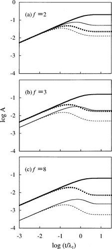
Time evolution of the anisotropies of Rouse–Ham eigenmode amplitudes during the creep process. Thick solid and dotted curves indicate the odd mode anisotropies, Aodd(t;1) and Aodd(t;2), respectively, and the thin solid and dotted curves show the even mode anisotropies, Aeven(t;1) and Aeven(t;2).
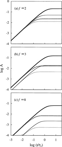
Time evolution of the anisotropies of Rouse–Ham eigenmode amplitudes after start-up of constant rate flow. Thick solid and dotted curves indicate the odd mode anisotropies, Aodd(t;1) and Aodd(t;2), respectively, and the thin solid and dotted curves show the even mode anisotropies, Aeven(t;1) and Aeven(t;2).
In both Figures 5 and 6, thick solid and dotted curves indicate the odd mode anisotropies, Aodd(t;1) and Aodd(t;2), respectively, and the thin solid and dotted curves show the even mode anisotropies, Aeven(t;1) and Aeven(t;2).
As noted from eqs 51 and 52, the growth of the anisotropy for respective eigenmodes under the constant-rate flow has a single characteristic time, τ/(2p−1)2 for p-th odd mode and τ/4p2 for p-th even mode. Correspondingly, the approach to the steadily flowing state (leveling-off of the plots shown in Fig. 6) is faster for higher order modes. These features indicate that respective eigenmodes behave as independent modes under the rate-controlled flow.
In contrast, during the creep process, the growth of the anisotropy of respective modes is associated with an infinite number of characteristic times λq; cf. eqs 49 and 50. Correspondingly, the anisotropy exhibits the overshoot except for the first mode (slowest odd mode; thick solid curve), and the steady state is attained simultaneously for all modes; see Figure 5. These features are a natural consequence of the interplay/correlation of the modes under the constant-stress requirement. The fast modes compensate for the slow growth of the anisotropy of the first odd mode at short t and thus all modes approach their steady state in a synchronous way. This compensation results in the overshoot of the anisotropy of the fast modes.
Finally, we turn our attention to a quantitative difference of the magnitude of interplay of the eigenmodes for the star chains with various f. This difference can be most clearly seen in Figure 7 where the anisotropies of the second odd mode and the lowest two even modes are normalized at their overshoot peaks and plotted against a reduced time, t/tpeak with tpeak being the time for the overshoot peak. The overshoot of these anisotropies is moderately enhanced with increasing f. This behavior is related to a relative decrease of the contribution of the even eigenmodes to S(n,t) with increasing f (compared to the odd mode contribution) noted in Figure 5 and eqs 49 and 50. The even modes of all orders p as well as the odd modes with p ≥ 2 exhibit the overshoot so as to compensate for the slow growth of the first odd mode, as explained above. Thus, the decrease of the even mode contribution requires the odd modes with p ≥ 2 and all even modes to make a larger compensation for the first odd mode, which results in the enhanced overshoot seen in Figure 7.
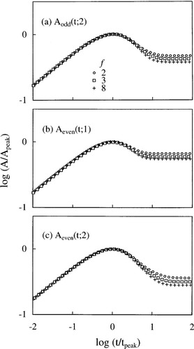
Comparison of overshoot of the anisotropies of low order Rouse–Ham eigenmodes during the creep process. The anisotropies for the star chains with various f are normalized at the overshoot peak.
CONCLUSIONS
We have solved the equation of motion for the Rouse–Ham star chains (in the continuous limit) to derive an analytic expression of the orientation function S(n,t) for the stress-controlled creep process. This expression indicates that the segments near the end of the star arm exhibit an overshoot of their orientational anisotropy to compensate for the slow growth of the anisotropy near the branching point and that the distribution of the anisotropy along the arm contour becomes more heterogeneous with increasing arm number f.
This interplay/correlation of the segments at different locations along the arm, not seen under the strain-controlled conditions, is a natural consequence of the requirement of the constant stress (constant total anisotropy) during the creep process. The corresponding interplay is noted for the Rouse–Ham eigenmodes: The odd modes with the order p ≥ 2 and all even modes exhibit the overshoot of their anisotropies to compensate for the slow growth of the anisotropy of the first odd mode. This overshoot is enhanced with increasing f.
These results demonstrate an important difference of the chain dynamics under the strain- and stress-controlled conditions. A rheo-optical experiment for partially labeled, non-entangled star chains enables us to examine this difference. This experiment is considered to be an interesting subject of future work.
Acknowledgements
This study was partly supported by Grant-in Aid for Scientific Research from JSPS (Grant Numbers 17350108, 17540381, and 17750204).
Appendix: APPENDIX A: TIME EVOLUTION EQUATION OF EIGENMODE AMPLITUDES
 (A1)
(A1) (t; q) and Ye (t; q) are the y components of the amplitude vectors B
 (t; q) and Be (t; q), respectively, and τ is the longest viscoelastic relaxation time of the Rouse–Ham star chain given by
 (A2)
(A2) (t; q) and Ḃe (t; q). However, making a sum of both sides of eq A1 for all f arms and considering eq 11, we find an equation that includes only Ḃe (t; q):
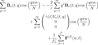 (A3)
(A3) (t;q):
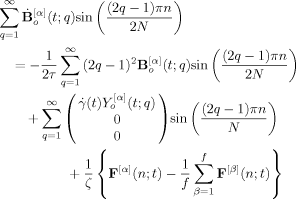 (A4)
(A4)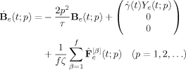 (A5)
(A5) (t; p)is p-th cosine-Fourier component of the Brownian force for β-th arm defined by
 (A6)
(A6)The x and y components of eqs A5 and A7, relevant to the calculation of the orientation function, are shown in eqs 13 and 14.
Appendix: APPENDIX B: CALCULATION OF DYADIC AVERAGES OF EIGENMODE AMPLITUDES
 (B1)
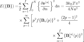
(B1) Ψ ({B}) d {B} = 1. From eqs 9–11, E is explicitly written in terms of {B} as3
 (B2)
(B2)Here, Be (p) and B (p), respectively, indicate the amplitude of p-th even and odd eigenmodes of α-th arm at equilibrium. Note in eq B2 that E is contributed from neither the cross-product between the even and odd modes Be · B
 (because the summation of B
 over α vanishes; cf. 11) nor the cross-products between the modes of different orders, B
 (p) · B
 (q) and Be (p) · Be (q) with p ≠ q (because these products vanish after the integration with respect to n.)
 BB′ Ψ ({B}) d {B}. Equations B1 and B2 immediately give
 (B3)
(B3) (B4)
(B4) (p) B
(p) B (q)〉, we need to consider a fact that the amplitudes for the f arms are not totally independent but correlated through eq 11. Following the argument by Zimm and Kilb,11 we can easily incorporate this fact in the calculation. They considered a pair of activated (correlated) arms, say α*-th and α**-th arms, that have B
 (p) = − B
 (p) to ensure the force balance at the branching point. The remaining arms are regarded as the uncorrelated arms. For the correlated α*-th arm, the summation term in eq B2, Σ
 {B
{B (p)}2, includes a term 2{B
 (p)}2 (because B
 (p) = − B
 (p)) thereby giving
 (B5)
(B5) (p)}2 and thus gives
 (B6)
(B6) (p) B
(p) B (q)〉 averaged over these probabilities are given by
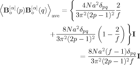 (B7)
(B7)(The same result can be obtained by explicitly utilizing eq 11 in eq B2, although this explicit method requires a lengthy integral calculation.)
Equations B4 and B7 indicate that the xy component of the dyadic average vanishes at equilibrium (〈X (p) Y
(p) Y (q)〉 = 〈Xe (p) Ye (q)〉 = 0), and this fact was utilized in derivation of eqs 23 and 24. The yy components of the averages at equilibrium are shown in eqs 25 and 26.
Appendix: APPENDIX C: STRAIN DURING THE CREEP PROCESS
 J(t) exp (−st)dt = σ
 ∫
∫ γ (t) exp (−st)dt:
 (C1)
(C1)Here, G̃(s) is the Laplace transformation of the relaxation modulus G(t) shown in eq 30. Note that eq C1 is equivalent to the linear viscoelastic relationship between G(t) and J(t),1 ∫ G(t − t′) J(t′)dt′ = t.
 (C4)
(C4) (C5)
(C5) (C6)
(C6) ) are obtained as
 (C7)
(C7) (C8)
(C8) (C9)
(C9) (C10)
(C10) { jq / λq} exp (− t/λ q) and thus its integral is given by
 (C11)
(C11) (C12)
(C12) (C13)
(C13)The strain rate obtained from this JR(t),
 , is utilized in eq 27 to calculate of the orientation function.
Appendix: APPENDIX D: ORIENTATION FUNCTION DURING THE CREEP PROCESS
Calculation of S(n,t)
 (D1)
(D1) S (n, t) exp (− st) dt, is explicitly obtained as
 (D2)
(D2)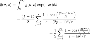 (D3)
(D3) (D4)
(D4) (D5)
(D5)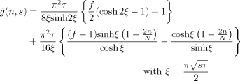 (D6)
(D6) / π2 τ, with φq being the eigenvalue determined by eq C6. The residues at these first order poles (=[(s − sq) S̃ (n, s)]
 ) are summarized as:
 (D7)
(D7) (D8)
(D8) (D9)
(D9)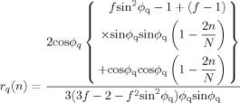 (D10)
(D10)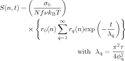 (D11)
(D11)Summation Rule for Eigenvalues
 :
:
 (D12)
(D12) (D13)
(D13)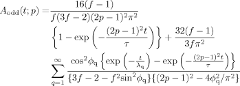 (D14)
(D14) (D15)
(D15) (D16)
(D16)(A special case of this rule for f = 2 was shown in the previous paper.4, 8)


 (t′; p) in eq