Multiple glass transitions and local composition effects on polymer solvent mixtures
Abstract
Recent differential scanning calorimetry (DSC) results on polystyrene–solvent mixtures show two distinct glass transitions whose positions and widths vary with composition. Parallel work on the dynamic response in polymer blends has focused on how segmental mobilities are controlled by local composition variations within a “cooperative volume” containing the segment. Such variations arise from both chain connectivity and composition fluctuations. We account for both using a lattice model for polymer–solvent mixtures that yields the composition distribution around polymer and solvent segments. Insights from our lattice model lead us to simplified calculations of the mean and variance of local composition, both in good agreement with lattice results. Applying our model to compute DSC traces leads to an estimate of the cooperative volume, since a larger cooperative volume both reduces the biasing effect of connectivity, and narrows the composition distribution. Comparing our results to data, we are able to account for the composition-dependent broadening with a cooperative length scale of about 2.5 nm. © 2006 Wiley Periodicals, Inc. J Polym Sci Part B: Polym Phys 44: 3528–3545, 2006
INTRODUCTION
Discussions of the glass transition of a polymer–solvent mixture typically assume the existence of a single glass transition temperature (Tg). Indeed, it is a traditional rule of thumb that samples exhibiting two Tg's are phase-separated. Yet polymer–solvent mixtures can often involve two components with widely separated glass transitions, implying very different segmental mobilities at any given temperature in this range. In addition, for such mixtures one expects that the average local composition around a segment will differ from the bulk. For the polymeric component there will be a local enrichment in self-composition because of chain connectivity. The impact of this effect on the glass transitions for a polymer blend was described some time ago by Lau et al.1 and Chung et al.,2 and quantified by Lodge and McLeish.3 Their arguments would evidently apply as well to the polymeric component in a polymer–solvent mixture.
For the small molecule component in a polymer–solvent mixture one can also argue for a shift in effective local composition relative to the bulk. If the environment around a polymeric segment has been enriched in polymer, it implies that the material still available to fill the rest of the cooperative volume around a segment of either type must be depleted in polymer. Thus the averaged local environment around segments of both types should be shifted relative to the bulk—but shifted in opposite directions. Both the local compositional difference as well as the aforementioned difference in component mobilities serve to accentuate the distinction between the two components, and support the notion that calorimetric measurements on polymeric mixtures should exhibit two glass transitions, reflecting two distinct local “points of view.”
In principle, therefore, at any given mixture composition one might expect two Tg's; however, only one is typically reported. For this reason a recent study by Savin et al.4 represents both an opportunity and a challenge. In their work Savin et al. presented and analyzed results on mixtures across the composition range of polystyrene (PS) with each of three substituted phthalates. Focusing, as did the authors, on PS/dibutylphthalate (DBP), we reproduce in Figure 1 their differential scanning calorimetry (DSC) traces for each of the pure components and for four mixture compositions. Note that two transitions are identified for the 30 wt % PS and 60 wt % PS compositions. In addition to the appearance of multiple transitions, we observe that the location of the transitions is clearly a function of composition for each component, and also that the DSC traces for each component in the mixture are broadened relative to the pure component trace.
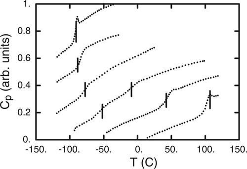
DSC data from ref.3. Traces shown are for PS-DBP mixtures with 0, 19, 39, 60, 80, and 100 wt % PS. Bars indicate the transitions as assigned by the authors. (Vertical offset is arbitrary.)
We have already discussed the origin of a local compositional average that is shifted relative to the bulk composition. Furthermore, note that use of such an average serves as a stand-in for the full composition distribution. Aside from the space that is occupied by segments that are covalently bonded to a central segment, we take the rest of the cooperative volume around the center to be filled randomly, reflecting the relative amounts of each species available. A distribution of local compositions implies a distribution of glass transitions, and this is the origin of increased broadening in the glass transitions for mixtures, relative to the transitions in pure components. Such a mechanism was proposed some time ago by Zetsche and Fischer.5
In this paper we propose a model that connects the broadening of the DSC results in the mixture to composition fluctuations around a polymer segment or a solvent molecule. Using a lattice approach, we show that by accounting for polymer connectivity and its effect on filling a specified local cooperative volume, the composition-dependent broadening can be predicted. We then distill these concepts and propose a route to the continuum analogue of the distribution of composition fluctuations, such that the breadth and positioning of the distribution reflect both the nature of the components and the dimensions of the cooperative volume.
In addition to the broadening of the DSC mixture traces, we are also interested in the composition-dependent positions of the transitions. A natural place to start our analysis will be the Lodge–McLeish (LM) model,3 the salient points of which are briefly reviewed here. Before proceeding, however, one might ask, Why not simply apply the LM model, modified to account for one component being a solvent, to the problem at hand?
Chief among the reasons for developing a new model is that the LM approach does not make predictions about the local composition distribution around a segment. It does predict the shift in the averaged local composition due to connectivity, but that alone would yield predictions for the mixture DSC traces which would be no broader than the pure component results.
Predicting the distribution of local compositions involves filling a “cooperative volume” around a given segment of interest, the dimensions of which should be on the order of a Kuhn length. In fact, the size of such a volume is an issue of current discussion. The analysis in the literature has centered around polymer blends and has focused on specifics relevant to NMR and dielectric relaxation data. Questions have been raised regarding the temperature dependence of this volume as the glass transition is approached. Some groups have looked at temperature dependence and by various routes have concluded that the cooperative length scale might increase by as much as a factor of 3 in going from well above Tg to near the glass transition. References 6 and 7 provide a good overview of this area.
It seems reasonable to take the magnitude of the cooperative volume to be intermediate, that is too large to be associated with the typical dimensions of a chemical repeat unit and likely too small to be represented as Gaussian strands. A lattice model is well suited to describe what might be happening on such a length scale. It also has the advantage of being easy to visualize, as well as allowing for analytic counting of configurations. Although the LM model does not incorporate all the features we appear to need, it does provide an important starting point in the consideration of how the mixture glass transitions depend on the averaged local composition. We therefore give a brief summary of the essentials here.
Lodge and McLeish describe a blend of two polymers A and B, which may in general have different Kuhn lengths and packing lengths. They consider the concentration within a cooperative volume VC of order the cube of the Kuhn length lK, surrounding a particular segment of polymer A. They observe that because of connectivity, the chain containing the particular segment will make a contribution ϕself to the volume fraction of A within VC.
They estimate ϕself = Ω/l , where Ω is the displaced volume of a polymer strand having an end-to-end length lK. Noting that the ratio Ω/l
 scales as the packing length lp, we see that ϕself scales as lp/lK. (The numerical coefficient depends upon the precise choice of VC and the definition of lp.)
 (1)
(1) (2)
(2) (3)
(3)The LM model is not bound to the Fox equation; other equations that provide a mixing rule for the composition-dependence of Tg could be used. However, the Fox equation has the advantage of requiring no adjustable parameters, and since the original LM paper made use of eq 3 we apply it here as well.
Our paper is arranged as follows. Under Description of Model, the lattice model is described in detail. Under Phenomenological Fits, we discuss fitting of the pure component DSC traces and characterization of the composition dependence of the experimentally recorded glass transitions. The section Comparison with Experimental Results comprises our applied results, wherein we compare our predictions for PS/DBP mixture traces with the experimental measurements, focusing on the impact of composition fluctuations on the breadth of the transition. We also consider the composition dependence of the mixture transitions, returning to the LM model and the Fox equation.8 Under the sections Self-Consistency and Lodge–McLeish and Alternative Estimate of Variance, we apply insights achieved from our lattice studies revisit the Lodge–McLeish model and to develop an alternative route for quantifying the effect of composition fluctuations, one which bypasses the lattice calculation of a composition histogram.
Under the last section, which is a summary and discussion of the work, we broach some of the larger issues that have arisen in the course of our studies, including those related to how ϕself is applied and understood, how our self-consistency arguments affect application of the LM model, and what our results imply about the cooperative volume at the glass transition. We conclude with some outstanding questions that we hope this work will prompt future studies to address.
RESULTS
Description of Model
To predict the effect of composition fluctuations on the breadth of the DSC transition, we model the solvent (A)–polymer (B) system on a Bethe lattice, or tree. Some advantages of using a tree lattice instead of an embeddable lattice, such as the simple cubic, are that every site has the same number of nearest neighbors (z) and no closed-loop configurations are possible. Figure 2 illustrates a z = 3 tree out to the third generation or “shell,” where we label the central site as the zeroth generation. Given a central site that is occupied by a segment of polymer, two of the sites in each subsequent generation must be filled with polymer connected to the central segment; this section of polymer is represented by the black segments in the figure. For simplicity, we choose the size of the lattice sites so that a solvent molecule occupies one lattice site.
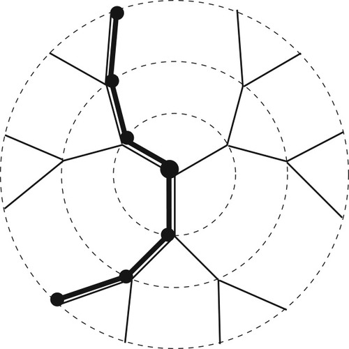
Schematic of a regular tree lattice (here z = 3 for illustrative purposes). Dashed circles indicate first, second, and third “shells” of lattice sites. Thick line indicates polymer configuration passing through central site.
 (4)
(4) such that they vanish whenever the variables take unphysical values, such as b > a or b < 0, and so forth. (Otherwise, we would have to take precautions when summing the probabilities over the range of values for the different indices, an issue that will become important later on.)
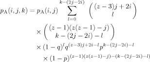
Filling of the second shell involves consideration of how the first shell is filled, given that for each unconstrained B segment in the first shell there must be two constrained B segments in the second shell. In addition, two of the second shell sites are filled with B segments which are connected through the first shell to the B in the zeroth shell. Thus the second shell contains 2i − 2 B segments that are constrained to be there. If we label the total number of B segments in the second shell as j, then the number k of unconstrained B's—that is, not connected to any B previously placed—which are next to a first shell B segment may have any value between 0 and j − (2i − 2).
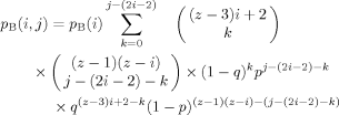
To determine the number of second shell sites open for filling, consider that each of the z first shell sites itself has z neighbors, z − 1 of which are in the second shell. However, each of the i − 2 unconstrained B segments in the first shell must be connected to two constrained B's in the second shell, and therefore has only z − 3 open neighbors in the second shell available for filling. In addition, the two constrained B's in the first shell are each connected to a constrained B in the second shell, and so each of these two first shell sites has only z − 2 open neighbors. Thus, the number of second shell sites that are neighbors to B-containing first shell sites is (i − 2)(z − 3) + 2(z − 2). In eq 5 below, the first binomial coefficient accounts for filling this set of open sites with the k unconstrained B segments that neighbor a first shell B, and the probability factor associated with this is (1 − q)k.
To determine the number of open sites remaining in the second shell, we note that each of the remaining z − i sites in the first shell has z − 1 second shell neighbors. Into this set we have yet to place the remaining B segments, that is, the j − (2i − 2) − k unconstrained B's that are neighbors to a first-shell A. The number of arrangements is given by the second binomial coefficient in eq 5, and the probability of finding this set of B's so placed is given by the factor of pj−(2i−2)−k. Here p is the probability of finding an unconstrained B segment next to an A segment.
Into the second shell sites that remain we place A segments. Recall that of the (z − 3)(i − 2) + 2(z − 2) open sites next to a first shell B, m are already taken by unconstrained B segments. Therefore the probability of finding A segments serving as neighbors of this set of first-shell B's is given by the factor q(z − 3)(i − 2) + 2(z − 2)−k. Finally, there are (z − 1) (z − i) – (j − (2i − 2) − k) neighbors to first-shell A's which are not already filled by unconstrained B's. The probability that these will be filled by A's is given by the factor (1 − p)(z − 1)(z − i) – (j−(2i − 2)−k). Such an accounting for the assignment of constrained and unconstrained sites is summarized in Table 1.
| A at Center | B at Center | |||
|---|---|---|---|---|
| Second Shell | Third Shell | Second Shell | Third Shell | |
| Constrained B sites | 2i | 2j − 2i | 2i − 2 | 2j − 2i + 2 |
| Unconstrained sites | ||||
| Total | z(z − 1) − 2i | z(z − 1)2 − (2j − 2i) | z(z − 1) − 2i + 2 | z(z − 1)2 − (2j − 2i + 2) |
| Neighbors of A | (z − 1)(z − i) | (z − 1)(z(z − 1) − j) | (z − 1)(z − i) | (z − 1)(z(z − 1) −j) |
| Neighbors of B | (z − 3)i | (z − 3)j + 2i | (z − 3)i + 2 | (z − 3)j + 2i − 2 |
 (5)
(5) (6)
(6) (7)
(7) (8)
(8) (9)
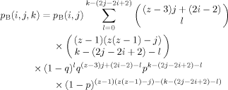
(9)There are still several steps required to translate from the probability results summarized in eqs 4–9 to a histogram representing a concentration distribution relevant for a given choice of the bulk composition. The result we need is the probability, given a B at the center of the tree, of finding a total of s B's in n shells (n = 1, 2, or 3), regardless of how they are distributed; we shall also need the analogous result for the case of an A at the center. These expressions are obtained by summing the relevant expression for the probability associated with the nth shell over the set of filling possibilities which are consistent with a total number of B (or A) segments equal to s. (Recall that we defined the binomial coefficients so that unphysical values of the indices lead to coefficient values of 0, allowing us to avoid thought-provoking constraints on the sums.)
 (10)
(10) (11)
(11)Here n is the number of shells in the cooperative volume, and Sn is the total number of sites in the first through nth shells. For our regular tree lattice S1 = z, S2 = z + z(z − 1), and S3 = z + z(z − 1) + z(z − 1)2.
In fact, before we can generate the numerical results for such a histogram we need to choose values for z, p, and q. We simplify the problem by observing that, since there is no special interaction between A molecules and B segments, the probability q of finding an A next to a B segment should be equal to (1 − p), the probability of finding an A next to another A. Similarly, the probability (1 − q) of finding an unconstrained B next to a B segment is equal to p, the probability of finding a B next to an A. Thus only one choice, say that of p, is required.
Naively, one might think that p should be set equal to ϕ, the bulk volume fraction of solvent; that is that any unconstrained site in our lattice should be filled from a reservoir of bulk material. However, because of the connectivity of the polymer as opposed to the solvent, when an unconstrained site in our lattice is filled with a B segment, it forces further sites in subsequent shells to also be filled with B segments. As a result, if we were to take p = ϕ, we would end up with too many B segments on the average in our configurations.
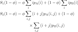
To make this more precise, we require a normalization condition, which may be used to determine the proper choice of p(ϕ). The condition is simply that the average number of B segments in any shell, averaged as well over what type of segment fills the central site, must equal 1 − ϕ (the bulk site fraction of B segments). The reason for this is that if we average over the filling of the central site, there is nothing special about the sites in any shell—they are just representative sites in the system.
 (12)
(12) (13)
(13)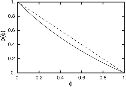
Shown is filling probability function p(ϕ) of eq 13 (solid curve) with 1 − ϕ (dashed line) for reference.
With an expression for p(ϕ) in hand, we can now compute the histograms hn,A(s) and hn,B(s), which give the probability of finding s B segments in the first through nth shells, with either an A or a B segment at the center. Figure 4(a,b) displays histograms hn,A(s) and hn,B(s) respectively, for n = 1, 2, and 3, and the value ϕ = 0.61. We plot the histograms as a function of s/Sn (recall Sn is the total number of sites in the first through nth shells; for z = 6, S1 = 6, S2 = 36, and S3 = 186).
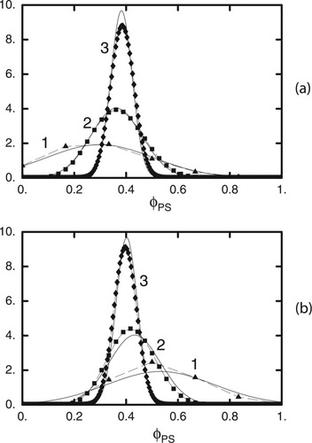
Histograms generated from our lattice model for case of 39% B (polymer), for first shell (triangles), second shell (squares), and third shell (diamonds). Solid curves are approximate Gaussian distributions described in the text. (a) A (solvent) at center. (b) B (polymer) at center.
Note that the peaks of the distributions are shifted away from 1 − ϕ = 0.39, particularly for smaller n values, for both A and B segments at the center. This shift is a consequence of connectivity constraints on the filling of the cooperative volume. When B is at the center, the shift is toward higher fractions of B; when A is at the center, the shift is toward lower B fractions (as we argued in the Introduction).
We also observe that the histograms narrow as the number of shells increases. This is expected, since with more independent choices as to the constituents, the fluctuations in the volume fraction decrease. Within the lattice model, varying the number of shells is comparable to varying the size of the cooperative volume in a continuum description such as the LM model. Similar results were obtained by Salaniwal et al. for the case of symmetric polymer blends, studied by lattice Monte Carlo simulations.9
Phenomenological Fits
The DSC traces of Figure 1 clearly exhibit two transitions at intermediate concentrations, for which the sample contains substantial amounts of both polymer and solvent. By observing the locations of the two transitions as a function of composition, it seems clear that the transition at lower temperature is an extension of the glass transition in the pure solvent, while the transition at higher temperature is an extension of the glass transition in the pure polymer.
In principle, we may expect that two transitions always contribute to the experimentally observed DSC traces of such polymer–solvent blends. However, depending on the difference between the pure component Tg's the contributions may overlay at intermediate compositions. At more extreme concentrations where the sample consists of mostly polymer or mostly solvent, only one transition is expected to be visible. We would like to separate the task of accounting for the location of these two transitions from the problem of describing the width of the two transitions. To do this we proceed as follows.
 (14)
(14)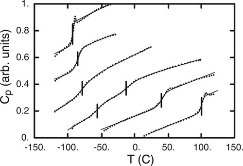
This procedure allows us to extract phenomenological values for the two glass transition temperatures Ts(ϕ) and Tp(ϕ), over much of the composition range. The results are shown in Figure 6. As is qualitatively evident in Figure 5, we see that the solvent glass transition depends only weakly on volume fraction, while the polymer glass transition is strongly dependent on the addition of plasticizing solvent.
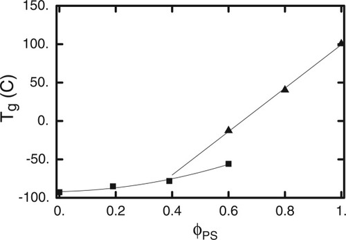
Fitted Tg's from Figure 5 plotted versus PS volume fraction. Squares denote lower transition (associated with DBP); triangles denote upper transition (associated with PS). Curves are least-squares fits to quadratic (for DBP) and linear (for PS) functions respectively.
To test the theory of the previous section, we first regard these transition temperature values as known, and focus on predicting the widths of the DSC traces. Later, we return to the question of predicting the composition dependence of the Tg's.
At the outset, we chose the lattice size to be such that a single solvent molecule fills one lattice site. Given the density and molecular weight of DBP (1.04 g/cm3 and 278.3 g/mol respectively), this implies that the volume of a lattice site is 0.443 nm3, corresponding to a cube 0.76 nm on a side. Given the density and molecular weight of PS (1.05 g/cm3 and 104.2 g/mol per monomer), we find that each lattice site can hold about 2.6 PS monomers. The characteristic ratio C∞ for PS is about 9.5, which can be interpreted as the number of monomers per Kuhn length. Thus each Kuhn segment of PS corresponds to about 3.7 lattice sites.
Comparison with Experimental Results
As a result of the efforts described in the previous sections we are now able to generate, for any bulk composition, distributions using one, two, or three lattice shells. In addition, we have experimental Tg's for the polymer for compositions ranging from pure to 60% PS and for DBP ranging from pure to 40% DBP. In what follows, we shall need Tg's for PS and for DBP for putative mixtures dilute in the respective component of interest. To estimate these, we extrapolate using our fits to data within the experimental range. Finally, we have also characterized each of the pure component DSC traces.
To generate DSC predictions, we sum the contributions from the trace associated with the PS transition and that associated with the DBP transition, weighting these contributions by the volume fractions of PS and DBP, respectively. The trace contributed by each component is obtained as follows. The component of interest is taken to occupy the center site (zeroth shell) and a histogram of local compositions is generated. Each composition in the histogram contributes a pure component trace. The transition of that trace is shifted to the glass transition appropriate for the composition and the height of the transition is weighted by the probability associated with that composition in the distribution. The set of weighted, shifted traces is then summed to give the overall trace for that component at that bulk composition. Finally, the overall traces for each of the two components (weighted by their respective bulk compositions) are summed to give the predicted DSC trace to be compared with experiment. For bulk compositions rich in one component the impact of the “dilute” trace will be negligible, and so only one transition will appear.
To determine the appropriate shifted Tg values as a function of the effective composition, we proceed as follows. We use our fits to the extracted values of Tg shown in Figure 6 to compute Tg for PS and DBP as a function of the bulk average composition. We then use the lattice model to compute the effective compositions in the vicinity of polymer and solvent as a function of bulk composition, from which Tg as a function of effective composition for polymer and solvent may be inferred.
In Figure 7 we compare our predictions with experimental data for four compositions ranging from 19 to 80% PS. The arrows on the figure indicate transition temperatures predicted using our fits to the experimental data (Fig. 6). At the lowest composition PS (19%) only the DBP transition (−85 °C) is observed and the predicted trace has a breadth which agrees well with that found experimentally. (Naïve extrapolation of the Tg–ϕ plot for PS would imply a PS transition near −140 °C, which is unreasonably low; however, within the calculation the contribution is so weak as to be undetectable.) For the 39% PS sample what we observe is evidently the overlay of the two transitions, as the temperatures are predicted to be at about −78 °C, within a few degrees of each other. The predicted trace captures rather effectively both the amplitude and the breadth of the transition. In the results for 60% PS the two transitions are clearly separated, that for PS occurring at −12.5 °C, and for DBP at −55.7 °C. This is the blend composition that shows most clearly the presence of two distinct transitions. We find very good agreement between predicted and experimental results, both for the amplitude and the breadth of each of the transitions. The last trace shows results for 80% PS. Here the PS transition at 40.3 °C is much stronger than the rather muted peak which, we predict, is associated with a DBP transition temperature of −26 °C. Once again, the predictions reproduce both the breadth and the rise found experimentally.
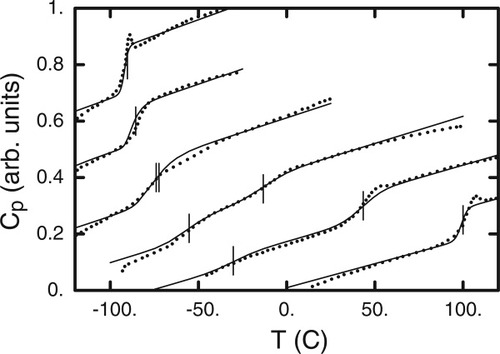
Lattice model predictions as described in text for DSC traces (solid curves), compared with data from ref.3.
The set of results summarized in Figure 7 provides evidence that our simple lattice model, applied using DSC results for the pure components, leads to predictions for the breadth and height of the mixture DSC traces that are in good to excellent agreement with that which is observed experimentally. It would therefore seem that the distribution of composition fluctuations predicted using the tree lattice is a reasonable approximate to what is being experienced by a segment of a given type in the real mixtures. However, there is one aspect to the analysis that has not yet been discussed.
Equation 10 shows that we have the flexibility to determine composition histograms accounting for one, two, or three shells of neighbors around a central segment. In generating the predictions shown in Figure 7 we obtain the best results by using two shells for the DBP predictions, and three shells for the PS predictions. Recall that Figure 4, which showed sample histograms associated with one, two, and three shells, illustrated the narrowing of the composition distribution as the cooperative volume around the central segment increased. In Figure 8 we show the DSC traces for each of the pure components, along with the respective traces for mixtures with 80% of each component. Consider the impact of adding 20% PS to pure DBP: Tg is hardly shifted at all, but the transition is considerably broader than that observed for pure DBP. This implies that local composition fluctuations are having a relatively large impact. On the other hand, when we turn to the two analogous traces for PS we see that, while the PS Tg is shifted significantly, the change in breadth of the PS transition in the blend is rather modest relative to that for pure PS. Given that the Tg for PS is apparently very sensitive to composition, this implies that local concentration fluctuations are having less impact on the PS experience in the blend. To model this, we need to consider a larger cooperative volume, hence the incorporation of the third shell. The choice of whether to incorporate two or three shells in generating model predictions has implications not just for the cooperative volume but also for the self-concentration of the species occupying the central segment. We turn to this issue in the discussion that follows.
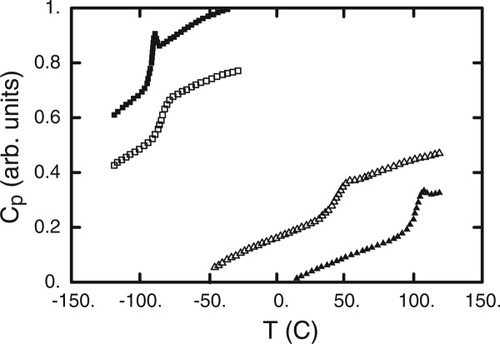
Shown are data of Figure 1, for pure PS (filled triangles) and 20% DBP (open triangles), and for pure DBP (filled squares) and 20% PS (open squares). Both transitions broaden upon blending, but the PS transition shifts much more in temperature than does the DBP transition.
Self-concentration and the Fox Equation
To this point we have not tried to predict the composition dependence of the glass transition. However, the appearance of two glass transitions and the implication of self-concentration as an important element lead naturally to consideration of the LM model. As summarized in the introduction, the LM model provides a route for predicting the composition dependence of two Tg's in a mixture. In their original paper an equation is given for the calculation of ϕself; however, in applications of the model by numerous groups this quantity has often been treated as an adjustable parameter. In a recent paper on the segmental dynamics of PS as the dilute component in a variety of solutions and blends, Lutz et al.10 summarize the results and observe that a considerable variation exists in the literature for ϕself of PS. However, they conclude that when the difference in Tg's between the two components is larger than 20 K or so, a single value of ϕself = 0.35 for PS appears to do remarkably well.
In Figure 9 we show that this value of ϕself does not account for the Tg results of the PS-DBP mixtures. The symbols represent the Tg values both for PS and DBP as a function of bulk composition, as reported by Savin et al. The upper curve in Figure 9(a) is the LM prediction for the composition dependence of Tg for PS using ϕ = 0.35. Although the composition range extends beyond the dilute limit as considered by Lutz et al. (which went up to 10 wt % PS in small molecule hosts), it is clear that the LM prediction using this value of ϕ
 does not match the data over any composition range. We also show the Tg data for DBP, along with the LM prediction using a ϕ
 = 0 for this small molecule component. Interestingly enough, although this curve fails to capture the solvent Tg behavior, it matches the PS data rather well. We pursue this in Figure 9(b), which shows the same two sets of experimental data along with LM fits to the PS results using ϕ
 = 0, 0.1, and 0.2. Also shown is a fit to the DBP results using ϕ
 = 0.42. The fact that the PS results are well-described using ϕ
 = 0 means that these data follow the predictions of the Fox equation, since the Fox equation is recovered in that limit. This should not be overinterpreted; as long as the cooperative volume is finite, ϕ
 cannot be strictly equal to zero. To emphasize this point, we also show the PS prediction using LM along with ϕ
 = 0.1, which is not too far off. However, the quality of the fit deteriorates as ϕ
 is increased, as illustrated by the curve obtained using ϕ
 = 0.2.
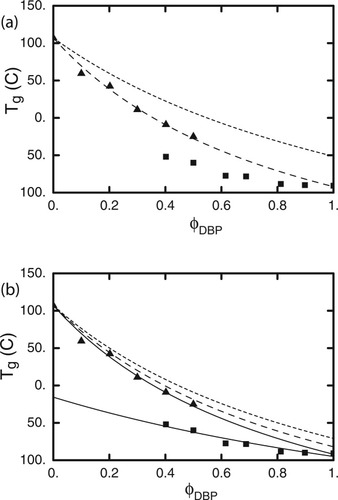
(a) Dotted curve is LM prediction of PS glass transition versus DBP fraction, assuming ϕself = 0.35; triangles are PS transitions. Dashed curve is LM prediction for DBP transition, assuming ϕself = 0; squares are DBP transitions. (b) Upper solid curve is LM prediction of PS glass transition versus DBP fraction, assuming ϕself = 0; dashed and dotted curves are for ϕself = 0.1 and 0.2 respectively; triangles are PS transitions. Lower solid curve is LM prediction for DBP transition, assuming ϕself = 0.42; squares are DBP transitions.
Before considering the implications of these results we wish to extend them by turning to a much older dataset for PS-solvent mixtures. Ferry11 summarized Tg values for PS in a wide variety of solvents, some of the studies being done over a considerable concentration range. In Figure 10 we replot these experimental Tg results for mixtures having up to 0.25 volume fraction of solvent. The form for the ordinate was chosen to yield a straight line with slope 1 − ϕself when plotting the LM equation, the limit of ϕ → 0 yielding the Fox equation. The lines are obtained by using values of ϕ
 equal to (from top to bottom) 0, 0.1, 0.2, and 0.35. It is clear that although a nonzero value of ϕ
 may be used, it must be small, certainly much smaller than 0.35.
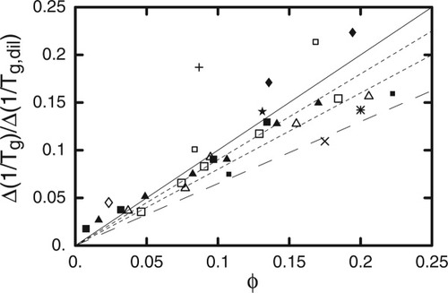
Symbols are glass transition data versus diluent fraction from Ferry (ref.11); different symbols correspond to different diluents, plotted as described in text. Solid line is Fox equation (LM with ϕself = 0); dotted lines are for ϕself = 0.1 and 0.2; dashed line is for ϕself = 0.35.
Self-Consistency and Lodge–McLeish
Our considerations of self-consistency between the filling of unconstrained sites and the overall average volume fraction of the two components are also applicable to the arguments leading up to the LM model for predicting the effect of the local environment on the Tg of a polymer segment.
Suppose for simplicity that the two polymers A and B in a blend have the same cooperative volume VC (i.e. the same Kuhn length), but different packing lengths and hence different values of ϕself. Consider the total number of pairs of A and B monomers such that the distance between them is less than the cooperative length scale. We may count this total number of pairs in two ways. We may either take the sum of the number of A segments within the cooperative volume of some B segment, summed over all B segments; or take an “A-centric” view, reversing the roles of A and B. Both procedures of course must give the same answer. This requirement turns out to constrain the way in which unconstrained sites are filled, such that eq 1 must be modified.
 (15)
(15) (16)
(16) (17)
(17) (18)
(18)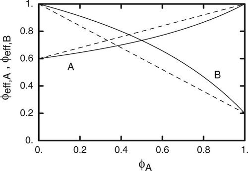
Solid curves are predictions from self-consistent LM eq 18 of ϕeff,A and ϕeff,B as functions of bulk ϕA; dashed curves are corresponding predictions of original LM. Here ϕself,A = 0.6 and ϕself,B = 0.2.
To see just how significant is the effect of an altered value for the effective volume fraction, we compute the Tg's of two hypothetical polymers A and B for which Tg,A = 200 K and Tg,B = 400 K. Figure 12 shows the predicted Tg's using the Fox equation with the effective volume fraction to predict Tg. It is worth mentioning here that taking the sum of the two resulting Tg's, weighted by the effective volume fractions, will yield a single Tg equal to what the original Fox equation would produce. This is just another way of showing that the effective volume fractions are self-consistent; following the same procedure using the original LM results would not produce the Fox Tg as a function of composition.
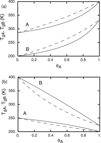
(a) Solid curves are predictions for polymer blends from self-consistent LM eqs 2 and 18 of Tg,A and Tg,B (i.e. with A and B at center site respectively) as functions of bulk ϕA; dashed curves are corresponding predictions of original LM. Here ϕself,A = 0.6 and ϕself,B = 0.2, Tg for pure A is taken to be 400 K and for pure B is 200 K. (b) As in (a), except that Tg for pure A is taken to be 200 K and for pure B is 400 K.
In fact, we can apply the result eq 18 to our lattice calculations. For this comparison, we need a value appropriate to the lattice model for ϕself,A and ϕself,B; we take ϕself,A = 0 and ϕself,B = 2n/Sn (the fraction of constrained segments connected to the B segment at the central site). Calculations of ϕeff,A and ϕeff,B using eqs 18 and 17 coincide with lattice results from eq 11. This agreement illustrates that the lattice model and the self-consistent version of the LM argument both properly account for chain connectivity even as it affects ϕeff of an unconnected species (solvent) in the presence of polymer.
Alternative Estimate of Variance
Thus far, we have computed histograms of volume fraction within the cooperative volume (represented within our lattice model as a number of shells in a tree) by essentially explicit enumeration. Now we consider an alternative approach to estimating the variance in effective volume fraction. In a recent work, Leroy et al. have treated the variance as a fitting parameter in accounting for the spectral width of dielectric relaxation data in polymer blends.12 However, Salaniwal et al.9 have addressed this problem by estimating variances in local composition using the random phase approximation (RPA) applied to the contents of a finite spherical volume. This yields an integral expression involving the RPA structure factor that must be evaluated numerically. Our simpler approach is based on the idea that the A and B segments pervading the cooperative volume have a typical size, and their presence or absence from the volume is determined by a set of independent decisions.
Consider the simplest case, that of a blend of two polymers A and B with the same packing length. Given a cooperative volume VC, a strand of either A or B pervading VC has some volume Ω. There are then some number n such strands required to fill VC. We may imagine filling VC by first generating configurations of the n strands, and then choosing among the n strands which are type A and which are type B. The volume fraction of A within VC fluctuates depending on how many A and B segments are chosen.
 (19)
(19) (20)
(20) (21)
(21)Thus the process of generating configurations may be regarded as a sequence of choosing either A (with some probability x) or B (with probability 1 − x), with their respective associated volumes inserted into the cooperative volume. As in the symmetric case described earlier, we simplify matters by taking a single, typical value for each of the inserted volumes ΩA and ΩB, although in the more precise lattice model ΩB would evidently vary among B strands.
 (22)
(22) (23)
(23) (24)
(24) (25)
(25) (26)
(26) (27)
(27) (28)
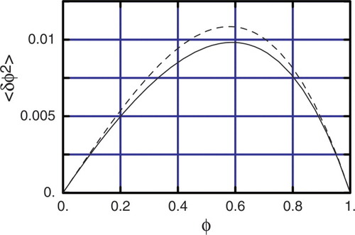
(28)We may compare the predictions of eq 28 to results from our lattice model, from which we can generate values of the variance in volume fraction as a function of composition. To use eq 28, we take ΩA = 1 (solvent occupies one lattice site) and VC = Sn (the total number of sites in the first through nth shells). Since ΩB varies in the lattice model, we retain it as a fitting parameter.
Figure 13 shows the variance computed from the lattice model for the second shell (VC = S2 = 36), and the prediction from eq 28 with ΩB = 2.04. Similarly good results are obtained for the first-shell variances with a slightly smaller value of ΩB = 1.45, and the third-shell variances with a slightly larger value of ΩB = 2.44.
Effective site fractions ϕeff,A and ϕeff,B versus ϕ for n = 1 (solid line), n = 2 (dashed line), and n = 3 (dotted line). Upper curves are ϕeff,B, lower curves are ϕeff,A. [Color figure can be viewed in the online issue, which is available at www.interscience.wiley.com.]
Thus this simple approximate approach to estimating the variance in volume fraction within the cooperative volume gives good agreement with the more involved lattice calculations, provided we use the volume per strand ΩB as a fitting parameter. The value of about two lattice sites for ΩB for the second shell is not unreasonable, given that only the longest central strand pervading the second shell is five segments long, those strands reaching into the first shell are just three segments long, and the strands reaching only into the second shell contribute but a single segment.
We can also compare the histograms computed from the lattice model to Gaussians with widths determined by eq 28 and mean positions determined by the self-consistent version of LM, that is eqs 18 and 17. To apply these equations to results of the lattice calculations, we take ϕself,A = 0 and ϕself,B = 2n/Sn (fraction of constrained segments arising from the central B site). In Figure 4, the solid lines correspond to Gaussians so determined, which are in good agreement with the lattice results.
In principle, this approach to estimating the variance in volume fraction could serve as a proxy for the lattice model histogram of volume fraction in generating DSC traces, by performing a sum of contributions to the overall trace over an appropriately discretized Gaussian distribution of effective volume fractions with the correct mean and variance. To pursue this would require a good a priori estimate of ΩB.
DISCUSSION
This paper deals with the impact of local environment on both the location and breadth of glass transitions in polymer–solvent mixtures. In the course of our studies we have had cause to examine critically notions about self-composition, the cooperative volume around a given segment, the impact of the packing length for a polymeric component, the utility of the Fox equation,8 characterization of composition fluctuations (using both a lattice model and a continuum description), and pitfalls in the LM model.3
As a starting point we focused on recent experimental DSC results for PS and DBP.4 We developed a simple tree lattice model as a means of computing the distribution of local environments around a segment in the mixture, which lead to the spread in Tg as reflected in the DSC results. A lattice description with chain connectivity naturally incorporates the effects of self-concentration associated with the presence of a polymeric component.13 It is less obvious that, having accounted for the self-concentration, scrupulous accounting is also required in filling the free space around such a segment (that is, the space not taken up by any covalently bonded segments) so as to yield the correct global average composition. This consistency condition turns out to require that the LM model be modified as well.
With our lattice histograms providing a means of accounting for local composition distributions, along with analysis of pure component DSC traces, we were able to predict the composition-dependent spread of the mixture DSC results. In doing so we required a means of calculating the shift in Tg expected for a given composition, which lead us both to apply and then ponder the form of the Fox equation. Finally, recognition that the lattice model is not a model of polymer solvent interaction or structure, but merely a mechanism by which a designated amount of space is to be filled by two different components, leads us to develop a simple continuum analogue. Our continuum description yields results that overlap those of the lattice approach, and under certain conditions, we believe it represents a clean route to accounting for local composition fluctuations.
The above-mentioned generalities are intended to give the casual reader a sense of the scope and depth of what we have covered in this paper. More detailed remarks follow.
General Principles
In this work, we have assumed that the contribution of a molecular segment within a polymer–solvent mixture to its glass transition is a function of the local concentration within some small cooperative volume containing the segment. To model this, we require a connection between the local concentration and the contribution of the segment to the glass transition, as well as a way of computing the distribution of local concentrations.
Within such a mixture, the average local polymer concentration in a small volume surrounding a polymer segment will be enriched relative to the bulk average, because of the connected polymer segments obliged to cohabit the volume.2, 4, 5 Likewise, the polymer concentration in a small volume surrounding a solvent segment will be depleted, because some of the polymer segments are bound to their connected brethren. These shifts in the effective concentration will lead to shifted glass transitions for two mixed components, relative to their locations if the local concentration were everywhere equal to the bulk value.
Beyond such effects of the average local concentration, there will be fluctuations in the local concentration around polymer and solvent segments. These variations in concentration, taken together with the concentration dependence of the Tg for each component, imply that the glass transition of each component will be broadened relative to its width in a pure sample.
Controlling both the shifts in the average local concentration and the breadth of the concentration fluctuations are two physical parameters: the size of the cooperative volume VC and the packing length of the polymer lp. As VC grows, the average local concentration approaches the bulk concentration and the fluctuations diminish. The packing length lp is a measure of the length scale over which a given chain makes a significant contribution to the local concentration. Bulkier and more flexible polymers have a larger packing length. Together, lp and VC determine ϕself, the self-concentration a polymer contributes in the vicinity of one of its own segments.
If we regard lp as a known material parameter and VC as a parameter to be determined by fitting to experiment, we see that VC can be determined in two ways: by choosing it so that the composition fluctuations give predicted widths of DSC traces that match experiment, or by choosing it so that ϕself in combination with eq 2 predicts the composition dependence of Tg. We shall return to this point shortly.
Our Lattice Model
We have developed a lattice description of the packing of polymer and solvent in a small volume, enabling us to compute the probability distribution of local concentration in a cooperative volume surrounding either a polymer or a solvent segment. A lattice model is simple to define, naturally contains short-distance cutoffs, and is amenable to enumeration. Use of a tree lattice eliminates polymer overlaps through avoidance of loops. Instead of the physical parameters VC and ϕself, we can choose the (integer) number of generations or “shells” in the tree lattice, and the (integer) coordination number of the lattice, as proxies for adjusting VC and ϕself.
Combining the above with a recipe for how the Tg of polymer or solvent depends on effective composition, as well as DSC data for the glass transition in pure polymer and pure solvent, we predict the shapes of DSC traces for polymer–solvent mixtures. These traces are the composition-weighted sum of contributions from the polymer and the solvent, each such contribution reflecting a different local composition distribution. We assume that each element of the distribution comprises the corresponding pure DSC trace for that component, shifted to its own local Tg, and having an amplitude proportional to mass fraction. We applied this recipe to the data on PS/DBP mixtures of Savin et al.4 with good results.
In generating the DSC traces we initially sidestepped the problem of predicting the dependence of Tg on effective composition by fitting the data of Savin et al. for Tg of each component as a function of bulk composition. We then used the lattice model to compute the effective compositions in the vicinity of polymer and solvent as a function of bulk composition, so as to translate from the bulk to the effective composition dependence of the experimental Tg values. As noted earlier, our analysis leads to two routes for the determination of VC. First, we adjusted the number of shells used in generating the DSC traces to give the best fit; this amounts to varying VC to control the composition fluctuations so as to match the widths of the DSC traces. Later, we determined values of ϕself that, when used with the LM prescription eq 2, gave reasonable fits to the Tg–composition data for the polymer and for the solvent. This amounts to adjusting VC (and hence ϕself) to match Tg(ϕ).
For PS solutions in DBP we found both the widths and the locations of the glass transitions associated with the PS component to be well-described by a small value of ϕself, of less than 0.1 or so. For the widths, we base this statement on the need to include up to n = 3 shells in our tree lattice to achieve a sufficiently narrow PS glass transition in the mixture. For the locations, this conclusion reflects the reasonable fit of eq 2 to the PS glass transition versus bulk composition with ϕself < 0.1. The significance of such a small value of ϕself relative to other published results is discussed toward the end of the paper.
Finally, in assuming random filling we are asserting that enthalpic interactions between segments are not strong enough to affect filling on the local scale. This is certainly true of polymer–polymer blends without strong attractions. It is even true of polymer blends near phase separation, because there χ is of order N−1 and so χ is a small effect on the scale of the Kuhn segment. However, for polymer–solvent blends the condition for phase separation is χ = 0.5, which is not small for effects on the scale of the Kuhn length. Thus for marginal solvents filling need not be random; such repulsive interactions would lead to concentration fluctuations that are enhanced beyond those for athermal solvents.
Comparison to Lodge–McLeish
Lodge and McLeish3 hypothesized as we have that the glass transition is a local phenomenon controlled by the concentration in a small cooperative volume VC surrounding a given molecular segment. LM assumed VC to be of order the Kuhn length cubed, though many subsequent workers have used ϕself and thus in effect VC as a fitting parameter. We have taken similar advantage, adjusting the number of shells in our lattice calculations to give a reasonable fit to the widths of DSC traces for the PS/DBP data.
LM adopted the Fox equation to compute the Tg for a segment from the local “effective” concentration. Initially, we extracted the dependence of Tg on composition from the DSC data itself; later, we followed LM and used the Fox equation, motivated by the observed concentration dependence of the polymeric glass transition in the PS/DBP mixtures.
The LM model makes a particular assumption about how the effective composition is enriched (eq 1). We have presented a self-consistent LM model, such that site-averaged effective compositions equal the bulk composition. This self-consistent LM model is in excellent agreement with results of the lattice calculations. Finally, no account is taken of concentration fluctuations in the LM model, and so it makes no prediction as to the broadening of glass transitions in polymeric mixtures.
Continuum Approach
We initially used the tree model to compute the composition distribution in a small volume of polymer solution. The filling of such a volume is the result of a number of independent decisions about the identity of segments occupying the space. This allows for an estimate of the variance of composition by elementary counting arguments.
Pursuing this approach, we developed a simple expression for the variance of composition that depends on knowing only the “typical” length of a polymeric segment within the cooperative volume. We showed that the composition distributions computed from the lattice model are well described by Gaussians constructed using the variance given by this argument eq 28, along with mean composition values given by our self-consistent form eq 18 of the LM model.
From this perspective the lattice model serves as a test bed to verify these routes to the effective composition, variance, and mean, and also as a way of computing the distribution of polymeric strand lengths within the cooperative volume. For the regular tree lattice with z = 6, it can be shown that the weight-averaged strand length 〈s〉 is independent of bulk composition, and approaches 7/3 ≈ 2.33 in the limit of a large number of shells (for n = 2, 〈s〉 = 2.19; for n = 3, 〈s〉 = 2.29). The vigorous branching of the regular tree leads to a preponderance of short strands.
One might expect that for a nonregular, space-filling tree the average strand length would be longer, which would mean that for a given size of VC the number of independently chosen segments filling VC would be smaller, and hence the composition fluctuations larger. We expect that for a more realistic (embeddable) tree lattice the required size of VC to match the width of the DSC traces would be somewhat larger than we found earlier.
Values of ϕself
As summarized earlier our results show that for PS solutions in DBP, both the widths and the locations of the glass transitions associated with the PS component are well-described by a small value of ϕself, of less than 0.1 or so. Correspondingly, we found it optimal to use three shells in modeling the polymer DSC transitions. We translate our result for the best-fitting number of shells in our lattice model into a size for the cooperative volume as follows. Since the tree lattice does not correspond directly to a compact, space-filling structure, we count the number of sites in the shells and convert this to a compact volume. Thus for the PS cooperative volume, which was best represented by n = 3 shells, we have 186 lattice sites, each site having a volume of one DBP molecule as described previously. The cooperative volume is thus estimated to be equivalent to a sphere of radius 2.6 nm.
This reflects a somewhat larger cooperative volume than has been found by other authors in analyzing results for PS solutions. In particular, Ediger and coworkers10 concluded that a value of ϕself of about 0.35 describes NMR segmental relaxation data for dilute PS solutions in various solvents. However, it must be noted that these data are limited by the frequency range of NMR to temperatures about 60 °C above the PS-related glass transition. Several authors have argued for an increase in the cooperativity length (i.e. the cube root of VC) as the glass transition is approached. This has recently been framed in the context of Adam-Gibbs theory, which describes the divergence of the cooperativity volume as the temperature decreases to somewhat below Tg.7
Here, we turn to estimate how large an increase in the cooperativity length is implied if we are to rationalize the present results with Ediger et al. At issue is how ϕself should scale with VC. If we assume that the polymer strand making the self-contribution is essentially straight, then ϕself should scale as V . If we instead assume that the polymer strand may be regarded as a random walk, ϕself should scale as V
 . (The latter scaling is consistent with the LM conclusion that ϕself scales as lp/lK.) If the polymer strand is “of the order of” a Kuhn length, the scaling is presumably in the crossover between these two limiting results.
The ratio of values for VC implied by two different values of ϕself could then be as large as (V′C /VC) = (ϕ′self/ϕself)3 (if random-walk scaling holds). Thus the linear dimension of the cooperative volume would be larger by a factor of at least (0.35/0.1) = 3.5 under the conditions of the DSC measurements (i.e. near to Tg) relative to the experiments of Ediger et al., 60 °C or so above Tg. This magnitude of increase in the cooperative length scale as temperature approaches Tg over such a range is not inconsistent with other published estimates.7
In contrast, the DBP glass transition varies only weakly with PS concentration; thus, when we fit to eq 2, a large value of ϕself,A (about 0.42) is required. Unlike our results for the PS transition, this is not consistent with the number of shells (n = 2) we found gave the best account of the DSC line shapes for the DBP transition. An apparent contradiction emerges: a large value of ϕself for DBP implies a very small cooperative volume (so that the single A site at the center dominates the concentration). But the relative narrowness of the DBP transition suggests a cooperative volume large enough so that composition fluctuations are somewhat suppressed.
In a very recent study Ediger and coworkers found that dilute tetracene in a variety of glass-forming hosts, including some that were polymeric, exhibited an effective glass transition that was equal to the matrix transition.14 However, these results were once again associated with NMR measurements, and the Tg's were extrapolated results from data that were collected at temperatures well above the transition. It may be that the Fox equation is not a good phenomenological description of the effect of local composition on the glass transition of small molecules. Or, perhaps a simplified lattice description of local composition fluctuations may be inadequate to describe molecules with a small cooperative volume. Or, “clustering” of the solvent molecules because of attractive interactions may lead to a larger ϕself. Clearly more work is needed to understand in detail the glass transition of the solvent in polymer–solvent mixtures. These issues may be confounded with the fact that the solvent is the low-Tg component in the Savin systems. It would be interesting to study a polymer–solvent system in which the polymer was the low-Tg component.
Remaining Questions
Several key questions remain unanswered. We have found that a larger cooperative volume for PS, hence a smaller value of ϕself, is required to fit the DSC data, because the experiment explores temperatures approaching Tg, rather than being limited to temperatures well above Tg as is the case for NMR studies, for example. This should be tested with other DSC studies, of mixtures of PS with other solvents. We would also expect that DSC studies of suitable polymer–polymer blends would show the effects of a larger cooperative volume, both in the location and breadth of observed transitions.
Use of the Fox equation to relate local composition to Tg remains ill-defended. It is curious that such a widely used expression should have such a murky provenance. We know of no derivation of the Fox equation in the literature. Indeed, the original reference8 is an abstract in the Bulletin of fthe American Physical Society, which does not give any theoretical argument for that particular form.
There are ambiguities as well regarding the classical literature data on PS–solvent mixture glass transitions, as summarized by Ferry.11 It is unknown whether these polymer–solvent mixtures exhibit two glass transitions in DSC traces; if so, it is unclear whether the single Tg's reported are to be associated with the polymer, or instead represent some weighted average of the transitions associated with the polymer and the solvent. At least on the polymer-rich end of the composition range, whatever transition was measured must be predominately related to the polymer.
So it is noteworthy that the data presented by Ferry is, while evidently scattered, reasonably consistent with the unmodified Fox equation, that is with small self-concentration for PS. It would be useful for a new and comprehensive set of data to be collected, given the PS/DBP results and emergence of a “local” view of the glass transition. Indeed, given the unresolved questions regarding ϕself and the cooperative volume, we believe it would be extremely useful to have new data that encompasses a set of glass-forming polymers spanning a range of packing lengths, dissolved in a variety of solvents.
Expanding the scope of miscible blend dynamics studies to polymer–solvent mixtures broadens the set of available systems for study. This work, which focuses on the glass transitions in PS DBP mixtures, presents new computational approaches through which the relationship between local segmental environments and dynamic heterogeneity may be clarified.
Acknowledgements
We thank Dan Savin and Tim Lodge for useful discussions, and we further benefited from Professor Savin's generosity in sharing unpublished data. J. E. G. Lipson acknowledges the support of the National Science Foundation [DMR-0502196].


