Free-breathing motion-informed locally low-rank quantitative 3D myocardial perfusion imaging
Funding information: Innosuisse - Schweizerische Agentur für Innovationsförderung, Grant/Award Number: 31010.1
Click here for author-reader discussions
Abstract
Purpose
To propose respiratory motion-informed locally low-rank reconstruction (MI-LLR) for robust free-breathing single-bolus quantitative 3D myocardial perfusion CMR imaging. Simulation and in-vivo results are compared to locally low-rank (LLR) and compressed sensing reconstructions (CS) for reference.
Methods
Data were acquired using a 3D Cartesian pseudo-spiral in-out k-t undersampling scheme (R = 10) and reconstructed using MI-LLR, which encompasses two stages. In the first stage, approximate displacement fields are derived from an initial LLR reconstruction to feed a motion-compensated reference system to a second reconstruction stage, which reduces the rank of the inverse problem. For comparison, data were also reconstructed with LLR and frame-by-frame CS using wavelets as sparsifying transform (-wavelet).
Reconstruction accuracy relative to ground truth was assessed using synthetic data for realistic ranges of breathing motion, heart rates, and SNRs. In-vivo experiments were conducted in healthy subjects at rest and during adenosine stress. Myocardial blood flow (MBF) maps were derived using a Fermi model.
Results
Improved uniformity of MBF maps with reduced local variations was achieved with MI-LLR. For rest and stress, intra-volunteer variation of absolute and relative MBF was lower in MI-LLR (±0.17 mL/g/min [26%] and ±1.07 mL/g/min [33%]) versus LLR (±0.19 mL/g/min [28%] and ±1.22 mL/g/min [36%]) and versus -wavelet (±1.17 mL/g/min [113%] and ±6.87 mL/g/min [115%]). At rest, intra-subject MBF variation was reduced significantly with MI-LLR.
Conclusion
The combination of pseudo-spiral Cartesian undersampling and dual-stage MI-LLR reconstruction improves free-breathing quantitative 3D myocardial perfusion CMR imaging under rest and stress condition.
1 INTRODUCTION
The clinical utility and value of dynamic contrast-enhanced myocardial first-pass perfusion imaging has been demonstrated in a number of landmark trials.1-3 While in today's clinical use, image data are mostly assessed visually or semi-quantitatively to identify ischemia, quantitative approaches4 have gained momentum with recent technical advances in data acquisition, reconstruction, and processing.5-8
In contrast to conventional dynamic multi-slice 2D imaging sequences, 3D approaches with whole-heart coverage allow data acquisition in a single time window per cardiac cycle.9 The potential clinical value of robust 3D myocardial perfusion imaging relates, in particular, to the ability to quantify the relative ischemic myocardial volume.10, 11 In view of the increasing utilization of ischemic burden as a marker for decision making for revascularization in stable coronary artery disease,12 added value has been indicated. Moreover, the importance of quantification of myocardial blood flow (MBF) and related parameters has been emphasized in the context of triple vessel coronary artery disease,13, 14 microvascular disease,15, 16 and other conditions.17
Dynamic 3D perfusion methods require substantial scan acceleration in order to accommodate data sampling into a sufficiently short acquisition window per cardiac cycle. To this end, k-t undersampling in conjunction with k-t BLAST, k-t SENSE,18-20 and k-t PCA21, 22 has initially been deployed and demonstrated in the clinical setting for various applications and compared against reference standards in single10, 11, 23-25 and multi-center trials.26, 27 Dedicated advances to improve the reconstruction accuracy from undersampled multi-slice 2D or 3D Cartesian,28-30 radial31-36 and spiral37-40 k-space trajectories have been proposed. Work on 3D Cartesian,22 radial stack-of-stars,41, 42 and spirals43 has demonstrated improvements with impact on quantitative perfusion parameters. The ramification of spatiotemporal fidelity on quantitative perfusion indices has been investigated and quantified.44
A challenge with k-t reconstruction, however, relates to the requirement to ensure sufficient spatiotemporal data correlations. Therefore, data acquisition is typically conducted in a breathhold, which has been limiting, in particular, during adenosine-induced stress. In order to increase patient comfort and compliance, initial research has been directed to enable free-breathing 3D data acquisition based on Cartesian30 and stack-of-stars undersampling.35
To address respiratory motion of free-breathing data acquisition, approaches applying global or local registration in the image domain have been described. To address challenges due to the dynamic contrast enhancement, image signal separation into low-rank and sparse components followed by model-based registration has been proposed.45 It is noted, however, that 2D registration-based methods can inherently only correct for in-plane and not continuous through-slice motion.
In addition to image-domain registrations, radial self-gating and respiratory motion binning have been used42, 46-48 to restrict or sort data to different respiratory states. However, retrospective binning of spokes into breathing and heart phases is only applicable for moderate undersampling or continuous acquisition schemes.42, 49
In general, nonrigid motion, corrupting the data, can be corrected for using an approximate solution given an estimated motion field.50 If rigid motion is assumed, it can be compensated for by application of linear phase shifts in k-space as demonstrated for perfusion imaging.51
Motion correction has become an important step to improve the conditioning of iterative image reconstruction methods.30, 52, 53 Block low-rank sparsity tracking (BLOSM) has proved beneficial,53 and has been extended to reconstruct from continuously acquired radial, simultaneous multi-slice, heart-phase resolved data.42 Similar methods have also been used in computed tomography perfusion imaging54 and in other MR applications such as MR parameter mapping55 and MR fingerprinting.56
For quantification of perfusion data, a dual-sequence, single-bolus approach is desirable.28, 41, 57 The arterial input function (AIF) is preferably recorded in the ascending aorta in an interleaved fashion.58
The present study proposes and validates a 3D motion correction approach for locally low-rank (LLR) image reconstruction of Cartesian pseudo-spiral in-out k-t undersampled single-bolus first-pass perfusion data. The method is referred to as respiratory motion-informed locally low-rank reconstruction (MI-LLR). It is shown that, by incorporating a transformation displacement field for each dynamic frame, MI-LLR is able to correct for non-rigid in- and through-plane organ motion during rest and stress. Numerical simulations and phantom experiments are used to demonstrate the robustness of the MI-LLR approach with respect to cardiac and breathing motion in comparison to LLR55 and frame-by-frame compressed sensing (CS) using wavelets as sparsifying transform (-wavelet)59, 60 reconstructions. In-vivo feasibility of the proposed method is assessed in subjects during rest and stress condition.*
2 METHODS
2.1 Image acquisition
A dynamically interleaved 2D/3D dual-sequence, single-bolus scheme was implemented on a clinical 1.5T MR system based on an electrocardiogram (ECG) -triggered saturation-recovery spoiled gradient echo sequences with T1- and B1-insensitive saturation preparation pulses62 as described previously.28
As shown in Figure 1A, the 3D perfusion scan is triggered to end systole. The 2D AIF images are acquired in the ascending aorta during diastole. A pseudo-spiral Cartesian undersampling pattern was implemented as illustrated in Figure 1B,C. The sampling distribution was defined by a variable density function63 with an elliptical k-space shutter as depicted in Figure 1B. For each dynamic imaging frame, k-space profiles were chosen according to the density distribution while avoiding profile duplication. At the k-space center, a 2 × 4 kz-ky area was fully sampled. The temporal order of profiles was according to a spiral-in—spiral-out scheme, placing the k-space center and the nominal saturation delay at half the acquisition time (Figure 1C). Imaging parameters were: TR/TE = 2.0/1.0 ms, spatial resolution: 2.5 × 2.5 × 10 mm3, FOV: 300 × 300 × 100 mm3, covering the full ventricle from apex to base, flip angle: 15°, acquisition window: 240 ms, saturation delay: 135 ms, undersampling factor R = 10.
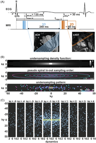
For the interleaved acquisition of the AIF, a fully sampled center-out Cartesian pattern was used with spatial resolution: 10 × 10 mm2, slice thickness: 15 mm, flip angle: 15°, acquisition window: 56–64 ms, saturation delay: 30 ms. TR and TE were set equal to the corresponding 3D sequence to avoid different T1 and T2* weightings.
All images were acquired on a 1.5T Philips Achieva MR system (Philips Healthcare, Best) using a five-element cardiac receive coil array. Gadobutrol (Gadovist, Bayer Schering Pharma) was used as contrast agent (CA).
2.2 Image reconstruction and motion compensation
Sensitivity maps for coil calibration were estimated from reference scans using the ESPIRiT method.69 Imaging data from the scanner were extracted and pre-processed using MRecon (Gyro Tools LLC).
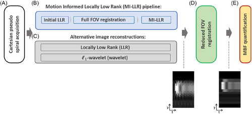
The entire framework is schematically outlined in Figure 2A–E. At first, data are acquired using the Cartesian pseudo spiral acquisition and put into the MI-LLR reconstruction, which encompasses two stages. In the first stage (Figure 2B), images are reconstructed using LLR (Equation 1) with a patch size of and underregularization to capture spatiotemporal image variations (). While the images show residual undersampling artefacts, motion patterns are not suppressed and visible. These images are registered using Equation (2) with regularization weight on the displacements to suppress the impact of residual aliasing artefacts in the initial LLR reconstruction. Thereafter, estimated displacement fields are used to perform the second stage of the MI-LLR reconstruction according to Equation (3), thereby allowing to reduce the regularization weight. The MI-LLR pipeline is illustrated for a representative case in Supporting Information Figure S1, which is available online.
For in-vivo image reconstructions, the minimum values of the regularization parameters and , which suppress background signal variation to 0.05% of the maximum image intensity, were chosen using a grid search approach and were and . The regularization parameter of the -wavelet reconstruction was set to 0.01. For synthetic experiments, optimal regularization parameters, yielding the lowest reconstruction error, were found using a grid search and were and .
2.3 Postprocessing and MBF quantification
Reconstructed 3D data were zero-filled to 1.25 × 1.25 × 5 mm3 and 2D-AIF images were zero-filled to 2.5 × 2.5 mm2. All image series were registered to compensate for residual motion prior to signal post-processing. Signal post-processing and perfusion quantification were conducted in Matlab (Mathworks). For local myocardial perfusion mapping, the images were convolved using the following kernel: to reduce noise at the cost of resolution.
The myocardium was segmented across the 10 slices and divided into six circumferential sectors per slice. Local and sector-wise myocardial signal time curves were derived along with the AIF.
2.4 Simulation studies
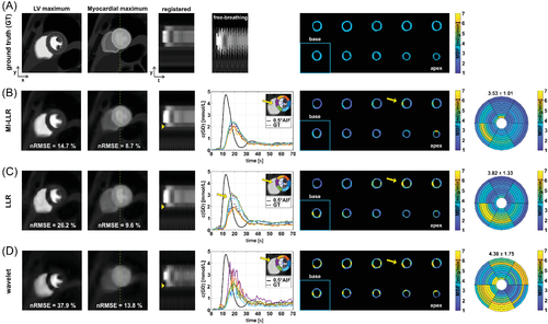
Numerical simulations were performed to validate the MI-LLR framework. A fully sampled free-breathing 3D perfusion numerical phantom was created using the signal model given in Equation (5) based on the MRXCAT simulation framework.76 Spatial resolution of the ground truth (GT) phantom was 1.25 × 1.25 mm2, slice thickness: 5 mm, 20 slices. To introduce partial volume effects, the GT object was subsequently downsampled to yield the final phantom parameters: 2.5 × 2.5 × 10 mm3, 10 slices, TR/TE: 2.0/1.0 ms, flip angle: 15°, CA dose: 0.075 mmol/kg body weight (b.w.), five receive coils, MBF: 3.5 mL/g/min, 70 simulated heart beats, R = 10. The numerical phantom was further modified to include cardiac and respiratory motion during readout to investigate the effects of motion on reconstruction and MBF estimation. Heart rates between 60 and 120 bpm and respiratory motion based on in-vivo navigator data with maximum amplitudes of 25 and 40 mm as provided in the supporting material (Supporting Information Figure S2) were simulated.
Statistical differences were assessed using the two tailed paired Student's t-test; p < 0.05 was considered significant.
2.5 Phantom studies
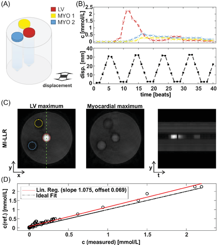
To verify the signal to concentration conversion after image acquisition and reconstruction, tubes were filled with purified water and doped with different concentrations of gadobutrol (from 0 to 2.25 mmol/L). The detailed setup of the phantom validation is summarized in Figure 5. The tubes were inserted into a cylindrical Agar phantom. Concentrations were sequentially varied to mimic the CA dynamics in the left ventricle and in myocardium by manually replacing tubes in between subsequent measurements. Concurrently, the phantom was displaced laterally to four positions with a maximum displacement of 30 mm to mimic in-vivo breathing motion dynamics.
2.6 In-vivo experiments
Twelve healthy volunteers (7 male) with an average age 25.2 ± 2.4 y underwent first-pass rest perfusion examinations; 7 underwent a rest and stress protocol. All volunteers were scanned upon written informed consent according to local ethics regulations. Two contrast-enhanced dual-sequence imaging experiments were run using CA boluses at doses of 0.075 mmol/kg b.w. to compare imaging at rest and stress. CA was injected at 4 mL/s and followed by a 30 mL saline flush at the same rate using a power injector (Medrad). Fifteen minutes were allowed for CA washout in-between the two bolus injections; stress imaging was always performed first. Adenosine (Kantonsapotheke, University Hospital Zurich) was injected for at least 3 min at doses of 140 μg/kg b.w./min under continuous monitoring of heart rate and blood pressure in accordance with standard clinical practice. Image acquisition covered 80 heartbeats during free breathing of the subject.
MI-LLR images, intensity-time profiles, concentration-time curves and resulting MBF maps were compared to LLR and -wavelet reconstructions for reference.
3 RESULTS
3.1 Simulation studies
Comparing MI-LLR to LLR and -wavelet reconstructions, image error was found to be reduced as shown by images at left-ventricular (LV) and myocardial (Myo) peak signal (Figure 3) with reconstruction nRMSEs for MI-LLR of 14.7% (LV) and 8.7% (Myo) versus LLR (26.2% and 9.6%) and -wavelet (37.9% and 13.8%). Intensity-time profiles indicate improved motion compensation with ML-LLR relative to LLR as indicated by yellow markers (Figure 3B,C). Concentration-time curves of the six sectors reflect improved motion compensation of the myocardium. In particular, septal sectors show reduced signal variance with MI-LLR when compared to LLR and -wavelet. For MI-LLR, local and sector-wise MBF maps reveal more uniform values of 3.53 ± 1.01 mL/g/min with MI-LLR when compared to 3.82 ± 1.33 mL/g/min with LLR and 4.38 ± 1.75 mL/g/min with -wavelet. MBF maps generally show MBF overestimation which is, however, reduced with MI-LLR when compared to LLR and -wavelet.
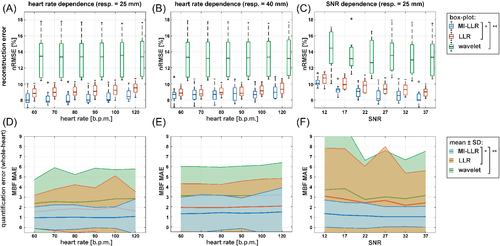
In Figure 4 reconstruction nRMSE and mean absolute error (MAE) of MBF as a function of heart rate, respiratory amplitude, and SNR are reduced with MI-LLR when compared to LLR and -wavelet. Heart rate dependencies for 25 and 44 mm peak respiratory amplitude show reduced reconstruction nRMSEs and MBF MAEs of MI-LLR when compared to LLR (Figure 4A,B,D,E). With a peak respiratory amplitude of 25 mm, median reconstruction nRMSEs for MI-LLR varied from 7.9% to 8.5%, while LLR shows higher median reconstruction nRMSEs (8.8%–9.5%), as does -wavelet (13.5%–13.4%). Reduced MBF MAEs resulted with MI-LLR (1.25–1.44) as compared to LLR (1.55–1.61) and -wavelet (2.39–2.86) up to a heart rate of 120 bpm. As summarized in Table 1, regional MBF showed significantly reduced variation with MI-LLR (±30%) as compared to LLR (±38%) and -wavelet (±45%). With a peak respiratory amplitude of 40 mm, MI-LLR yielded reduced median nRMSEs of 8.7%–8.9% when compared to 8.8%–9.3% for LLR and 13.1%–13.2% for -wavelet; reduced MBF MAEs are seen with MI-LLR (1.25–1.44) when compared to LLR (1.89–2.03) and -wavelet (3.05–3.14). Regional MBF showed significantly reduced variation for MI-LLR (±38%) when compared to LLR (±44%) and -wavelet (±44%). The SNR dependence demonstrates improved performance of MI-LLR when compared to LLR; median reconstruction nRMSEs decreased from 10.1% to 8.1% for MI-LLR when compared to 10.8%–9.0% for LLR, and 14.5%–13.4% for -wavelet when increasing SNR from 12 to 37 (Figure 4C); likewise reduced MBF MAE is seen with MI-LLR (1.38–1.07) when compared to LLR (3.11–2.44) and -wavelet (3.73–3.17) with reduced regional MBF variation for MI-LLR (± 34%) as compared to LLR (± 53%) and -wavelet (± 52%).
| MBF quantification metrics | Motion-informed locally low-rank (MI-LLR) | Locally low rank (LLR) | -wavelet (wavelet) | ||
|---|---|---|---|---|---|
| Simulation | mean MBF ± SD [ml/g/min] (SD [%]) (ground truth = 3.5 ml/g/min) | Resp. amplitude: 25 mm, HR: 60–120 bpm | 3.44 ± 1.03 (30%)*, ** | 3.77 ± 1.43 (38%)*, ** | 4.04 ± 1.82 (45%) |
| Resp. amplitude: 40 mm, HR: 60–120 bpm | 3.74 ± 1.42 (38%)*, ** | 3.67 ± 1.62 (44%)*, ** | 4.59 ± 2.02 (44%) | ||
| Resp. amplitude: 25 mm, SNR: 12–37 | 3.43 ± 1.17 (34%)*, ** | 3.96 ± 2.10 (53%)*, ** | 4.44 ± 2.31 (52%) | ||
| In-vivo | Stress: ± mean intra-volunteer SD [ml/g/min] (SD [%]) | Mean resp. amplitude ± SD: 24.9 ± 7.4 mmMean HR ± SD: 87 ± 9 bpm | ±1.07 (33%)** | ±1.22 (36%)** | ±6.87 (115%) |
| Rest: ± mean intra-volunteer SD [ml/g/min] (SD [%]) | Mean resp. amplitude ± STD: 16.3 ± 9.3 mmMean HR ± SD: 67 ± 7 bpm | ±0.17 (26%)*, ** | ±0.19 (28%)*, ** | ±1.17 (113%) | |
- Note: Significant differences (p < 0.05) of absolute and relative MBF SD (SD [%]) are marked by asterisks:
- * Refers to significant differences when MBF SDs of motion-informed locally low-rank (MI-LLR) are compared relative to LLR.
- ** Refers to significant differences when MBF SDs of MI-LLR or LLR are compared relative to -wavelet (wavelet). In-vivo SDs were normalized by the means (SD [%]).
The average motion accuracy after the final registration step was 1.96 and 2.18 mm for 25 and 40 mm breathing amplitude, respectively. After registration, differences in motion accuracy between MI-LLR and LLR were insignificant.
3.2 Phantom studies
Reconstruction results for the proposed method are shown in Figure 5. Exact signal to concentration conversion is examined by comparison of reference to measured concentration with a linear regression model. Figure 5D shows the CA concentrations derived from T1 values measured with the proposed 3D acquisition and reconstruction. Data are in agreement up to gadolinium concentrations of 2.4 mmol/L as indicated by the slope of linear regression of 1.08 (offset = 0.07).
3.3 In-vivo studies
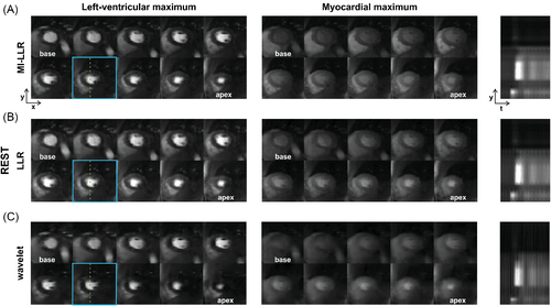
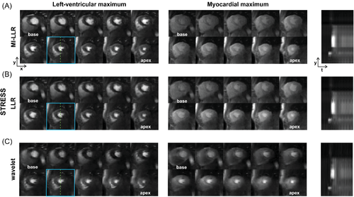
In Figures 6 and 7, example reconstruction results for rest and stress acquisitions of a healthy male volunteer (average heart rate 70 bpm [rest] and 81 bpm [stress], navigator displacement 20 mm [rest] and 24 mm [stress]) are reported at peak LV and myocardial contrast maximum, and intensity profiles (videos are included as Supporting Information Videos S1 and S2). At rest, MI-LLR images appear less blurred than LLR at myocardial intensity maximum. Intensity profiles indicate sharper borders between myocardium and blood pool for MI-LLR when compared to LLR. At stress, MI-LLR images appear less blurred than LLR; -wavelet images show pronounced artefacts. Intensity profiles indicate sharper borders between myocardium and blood pool for MI-LLR as compared to LLR images, with more residual motion seen in the LLR profile, while -wavelet intensity profiles are dominated by pronounced signal intensity artefacts.
In Figures 8 and 9, corresponding quantifications are summarized at rest and stress, respectively. At rest, concentration-time curves show residual artefacts for both MI-LLR and LLR. Concentration time curves exhibit reduced fluctuations over time for MI-LLR (signal maximum at 0.47 mmol/L with 0.30 ± 0.06 mmol/L) when compared to LLR (signal maximum at 0.58 mmol/L with 0.32 ± 0.08 mmol/L). Concentration time curves from -wavelet reconstructions are corrupted by artefacts. Rest maps show uniform MBF values but signal spilling in the basal slices. Apical locations show reduced local MBFs as compared to basal locations. MBF variation are reduced using MI-LLR (±0.11 mL/g/min) vs. LLR (±0.13 mL/g/min) versus -wavelet (±0.27 mL/g/min).
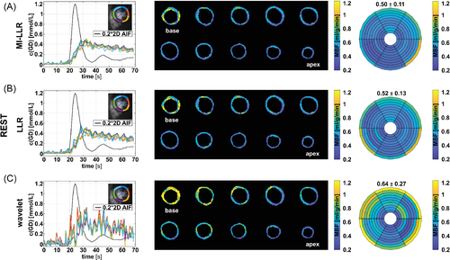
At stress (Figure 9), concentration-time curves show residual artefacts induced by motion for both MI-LLR and LLR. Signal maxima are lower for MI-LLR (at 0.69 mmol/L with 0.65 ± 0.05 mmol/L) as compared to LLR (at 0.80 mmol/L with 0.69 ± 0.08 mmol/L). MBF maps show uniform MBF values but signal spilling in the basal slices. Apical locations show reduced local MBFs as compared to basal locations. Bulls eye plots indicate that regional means are compromised less with MI-LLR; MBF variation is seen to be significantly reduced (p < 0.05) using MI-LLR (±0.70 mL/g/min) vs. LLR (±0.79 mL/g/min) versus -wavelet (±3.36 ml/g/min).
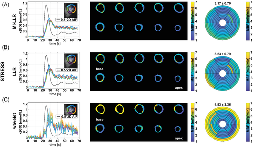
Spatial variation of CA concentration across the myocardium at peak myocardial enhancement for all volunteers is compared in Supporting Information Table S1. MBF quantification results for all subjects are summarized in Table 1 and Supporting Information Figure S3. One subject showed a high response to adenosine stress resulting in heart rates exceeding 130 bpm. Failing ECG gating resulted in triggering of only every second heartbeat. The stress scan was thus excluded from analysis. For MI-LLR reconstruction, at an average resting heart rate of 67 ± 7 bpm, the average inter-volunteer MBF was 0.65 ± 0.22 mL/g/min, while, under stress and an average stress heart rate of 87 ± 9 bpm, the average MBF was 3.23 ± 0.61 mL/g/min compared to 0.68 ± 0.23 mL/g/min (rest) and 3.39 ± 0.34 mL/g/min (stress) for LLR versus 1.03 ± 0.75 mL/g/min (rest) and 5.94 ± 3.98 mL/g/min (stress) for -wavelet. Intra-volunteer variation of absolute and relative MBF was lower in MI-LLR (±0.17 mL/g/min [26%] and ±1.07 mL/g/min [33%]) versus LLR (± 0.19 mL/g/min [28%] and ± 1.22 mL/g/min [36%]) and versus -wavelet (±1.17 mL/g/min [113%] and ±6.87 mL/g/min [115%]), for rest and stress, combined. At rest, the reduction in regional MBF variation between MI-LLR and LLR was significant (p = 0.0073); at stress it was insignificant. SDs of MBF values derived from MI-LLR and LLR were significantly reduced when compared to -wavelet at rest and stress.
4 DISCUSSION
In this study, a 3D motion-informed locally low-rank image reconstruction framework, combined with Cartesian pseudo-spiral k-t undersampling, was developed and the suitability for robust free-breathing whole-heart quantitative perfusion imaging has been demonstrated under rest and stress conditions in volunteers.
The proposed MI-LLR approach yields qualitative and quantitative improvement compared to LLR reconstruction for free-breathing imaging. In-vivo MBF values derived from both 3D MI-LLR and LLR agree with the range of values reported for quantitative 2D perfusion CMR methods.17 Reduced variation of regional MBF values was found for MI-LLR when compared to LLR and -wavelet in simulation and for in-vivo data at rest. Average rest and stress values and their variations compare well to data from other 3D studies.28, 42, 44 Differences between MI-LLR and LLR depend on individual subjects' breathing pattern and heart rates (example cases shown in Supporting Information Figures S5–S8; Supporting Information Videos S3 and S4).
Especially in simulation, MI-LLR reduces signal elevations in the septal region as caused by high contrast signal from the right-ventricular and LV blood pools. The visually apparent trend for underestimation in the infero-lateral regions is relative to the sites of increased signal which are observed predominantly in basal slices.
In order to relate MI-LLR and LLR to methods commercially available on clinical MR systems, frame-by-frame compressed sensing with wavelets as sparsifying transform and coil encoding was used, which resulted in significant image distortions and erroneous MBF quantification. The Cartesian pseudo spiral in-out sampling pattern used in the present work ensured that the central k-space was always covered halfway during the acquisition window. This differs from other work that promotes motion robustness by means of radial sampling strategies,41, 42, 77 where the central k-space is traversed by every profile and as such is susceptible to variations in motion state throughout the acquisition, unless this is accounted for by, for example, retrospective binning. Of note, 3D stack-of-stars acquisition schemes inherently demand higher undersampling factors, i.e., pi/2 more data is required in order to fulfil the Nyquist criterion when compared to Cartesian sampling.9, 41 Possible reduction of the acquisition window by means of partial echo and partial Fourier sampling as used in other studies28, 41 was avoided as the approximated Hermitian symmetry is potentially violated by the local modulation of signal phase due to the CA.78 However, cardiac motion during the acquisition could have contributed to Gibbs ringing, i.e., dark-rim artefacts,79 which were observed in some cases in this study (e.g. Supporting Information Video S2).
Conversion of signal intensities to concentrations requires a signal model. Phantom validation (Figure 5) of MI-LLR signal intensity to concentration conversion showed good agreement within precision of experiment in the range of expected myocardial gadobutrol concentrations from 0.1 to 2.3 mmol/L and motion amplitudes of 30 mm.
Simulation studies using the MRXCAT framework confirmed sufficient robustness of MI-LLR at higher heart rates and breathing amplitudes and was shown to outperform LLR and -wavelet over a realistic SNR range. MBF quantification from MI-LLR reconstruction showed reduced variability in apical and basal sectors, as well as reduced overestimation of midventricular, infero- and anteroseptal regions. The investigated respiratory amplitudes of 25 and 40 mm in feet-head direction were taken from recorded in-vivo respiratory motion amplitudes as shown in Supporting Information Figure S2; other work only considered amplitudes of 1.7 and ∼8 mm.30, 42 In the simulation studies, sinusoidal breathing patterns of 4.5 s cycle duration were assumed; especially under stress, more irregular and abrupt breathing patterns might occur. In these cases, the exact implications of sudden motion on quantification accuracy remain to be quantified.
It is noted that the perfusion model (Equation 7) fitting problem is reasonably well posed, i.e., three model parameters are fitted considering approximately 40 time points per pixel (the exact value depends on the time span of the first pass and thus the shape of the curve). Therefore, no clear trend in MBF accuracy vs. heartrate or SNR could be detected, contrary to reconstruction nRMSEs (Figure 4A–C). However, systematic bias is intrinsic to each of the considered methods; therefore, a significant improvement of MI-LLR compared to LLR in terms of MBF accuracy was seen in the simulation studies. In the future, a blood tissue exchange model (BTEX) with four free parameters modelled as partial differential equations should be tried as proposed in other work.80, 81 In that case, superiority of MI-LLR motion compensation is expected to improve quantification robustness more profoundly than shown for the Fermi-based fitting.
In image reconstruction, the patch size as well as the range of regularization parameters were determined empirically and found to be generalizable to all datasets. A reference ground truth image could alternatively be used to optimize s, 82 the acquisition of which is, however, hampered by the residual CA in the tissue and the resulting change in contrast. The effects of regularization and image registration used on net spatiotemporal resolution are yet to be determined. Although simulation and in-vivo results show motion robustness of the proposed reconstruction, maximum scan acceleration factors to reduce the influence of intra-shot cardiac motion contributions remain to be investigated. Previous work exploiting motion information for 3D perfusion imaging utilized uniform Cartesian k-t undersampling30 in conjunction with based regularization, as opposed to non-uniform k-t undersampling and nuclear norm regularization used here. As a result of -regularization, temporal blurring was observed compromising MBF quantification.30 A comparison of different quantitative free-breathing perfusion approaches (i.e., data acquisition, reconstruction and MBF quantification) for uniform Cartesian, random Cartesian, radial, and spiral undersampling based on synthetic data could be beneficial and will be subject of future work.
Relating to previous work that uses motion correction with LLR, the BLOSM approach is similar to the proposed MI-LLR strategy but was only applied in the context of 2D data53; through-plane motion from true 3D acquisitions was not investigated. Continuous Radial Interleaved simultaneous Multi-slice acquisition at sPoiled steady-state (CRIMP) achieves whole-heart coverage combining self-gating and patch tracking in a continuous multiband acquisition, which uses dual bolus injections for MBF quantification.42
Computation times for the entire reconstruction were on the order of ∼15 min per scan using a hybrid CPU-GPU implementation. Processing times are mainly determined by the cost of the 3D image registration steps. Furthermore, currently a five-channel coil is used. For larger numbers of receiver channels, the proposed method could be adapted using coil compression methods.83
A limitation of our study is the small number of subjects included. In order to allow for more generalizable statistical results, future studies should enroll larger numbers of subjects without and with suspected coronary artery disease. Diagnostic accuracy should then be addressed in simulation and the in-vivo evaluation. Reader assessment regarding image quality should be investigated. The method was implemented at 1.5T but is applicable to other field strengths.
5 CONCLUSIONS
The combination of 3D Cartesian pseudo-spiral in-out undersampling in conjunction with motion-informed low-rank reconstruction improves single-bolus free-breathing quantitative 3D myocardial perfusion imaging under rest and stress condition.


