Prediction of residence time distribution of a single-screw rubber extruder by parameterizing the transfer function using experimental data
Vorhersage der Verweilzeitverteilung eines Einschnecken-Kautschukextruders durch Parametrisierung der Übertragungsfunktion anhand experimenteller Daten
Abstract
enWith the ongoing digitalization in the industrial sector, also called Industry 4.0, automation techniques offer huge potential for the rubber industry. Advanced automation methods allow for precise control of the extrusion process and increase the consistency in product quality. Since product quality is affected by process parameters in a complex way, predicting the flow conditions, the thermal conditions and the mixing in an extruder is a prerequisite for more sophisticated Industry 4.0 applications. These Industry 4.0 applications require short computing times and thus sufficiently fast models for online implementation in production systems. A useful measure for the flow inside the extruder is the residence time distribution. It enables an analysis of the residence time of the material particle in the process and subsequently a statement about the mixing characteristics. For the investigation of the residence time distribution and the effect of process parameters on residence time properties, a single-screw rubber extruder equipped with a gear pump was used. In this contribution, we present a method to identify the residence time distribution for a certain compound using experiments. We describe an experimental procedure with a special tracer material and a modified image processing method to identify the residence time distribution. The experimental data and analyses, in particular, the input and output signals of the experiments, are used to determine the residence time distribution (transfer function) of the system. Based on previous findings from literature and experimental studies of the process, the influences of selected parameters on the transfer function were investigated and used to parameterize a general transfer function for the chosen compound. Consequently, the derived transfer function is used to predict the residence time distribution of the process and the results are validated with experimental data. We discuss the potential of the method for an online implementation in a production system and outline how this method can be used within predictions for advanced process control.
Translation abstract
deMit der fortschreitenden Digitalisierung im Industriesektor, auch Industrie 4.0 genannt, bieten Automatisierungstechniken ein enormes Potenzial für die Kautschukindustrie. Fortschrittliche Automatisierungsmethoden ermöglichen eine präzise Steuerung des Extrusionsprozesses und erhöhen die Konstanz der Produktqualität. Da die Produktqualität in komplexer Weise von den Prozessparametern beeinflusst wird, ist die Vorhersage der Fließbedingungen, der thermischen Bedingungen und der Vermischung in einem Extruder eine Voraussetzung für anspruchsvollere Industrie 4.0-Anwendungen. Diese Industrie 4.0-Anwendungen erfordern kurze Rechenzeiten und damit ausreichend schnelle Modelle für die Online-Implementierung in Produktionssystemen. Ein nützliches Maß für die Strömung im Extruder ist die Verweilzeitverteilung. Sie ermöglicht eine Analyse der Verweilzeit der Materialpartikel im Prozess und damit eine Aussage über das Mischungsverhalten. Für die Untersuchung der Verweilzeitverteilung und der Auswirkung von Prozessparametern auf die Verweilzeiteigenschaften wurde ein Einschnecken-Kautschukextruder mit einer Zahnradpumpe verwendet. In diesem Beitrag stellen wir eine Methode zur experimentellen Identifizierung des Verweilzeitverteilung für eine bestimmte Verbindung vor. Wir beschreiben ein experimentelles Verfahren mit einem speziellen Tracer-Material und einer modifizierten Bildverarbeitungsmethode zur Identifizierung der Verweilzeitverteilung. Die experimentellen Daten und Analysen, insbesondere die Eingangs- und Ausgangssignale der Experimente, werden zur Bestimmung der Verweilzeitverteilung (Übertragungsfunktion) des Systems verwendet. Basierend auf früheren Erkenntnissen aus der Literatur und experimentellen Untersuchungen des Prozesses wurden die Einflüsse ausgewählter Parameter auf die Übertragungsfunktion untersucht und zur Parametrisierung einer allgemeinen Übertragungsfunktion für die gewählte Verbindung verwendet. Folglich wird die abgeleitete Übertragungsfunktion zur Vorhersage der Verweilzeitverteilung des Prozesses verwendet und die Ergebnisse werden mit experimentellen Daten validiert. Wir erörtern das Potenzial der Methode für eine Online-Implementierung in einem Produktionssystem und skizzieren, wie diese Methode im Rahmen von Vorhersagen für eine fortschrittliche Prozesssteuerung verwendet werden kann.
1 Introduction
The extrusion process is a core process for the processing of rubber and rubber compounds. A central challenge in the management of elastomer extrusion processes is the optimal choice of production parameters and raw materials for elastomer compounds to ensure consistent product quality at maximum throughput. This requires a high level of expert knowledge and elaborate testing procedures. Since the quality of the product is influenced by the process parameters, the analysis of the residence time of the extrusion process and subsequently the homogenization behaviour is of high significance. For example, homogeneity and cross-linking behaviour strongly depend on how long the rubber compound is exposed to the prevailing process parameters. In addition, the undesired cross-linking of material mixture within the extrusion process can be attributed, among other things, to the residence time behaviour.
Prior research has focused on determining the residence time distribution of different types of extruders, such as single screw extruders, co-rotating twin screw extruders or buss kneaders for the extrusion of various materials, such as plastics and in the field of food engineering 1-18. Three main approaches have crystallized: the off-line method, the in-line method and the on-line method 1, 4-8, 13, 15, 16, 19-26.
In the field of rubber extrusion, the mentioned methods have not yet been sufficiently investigated or implemented. The digital image processing method is an off-line measurement method for the residence time distribution of an extrusion process from the field of plastics and food extrusion 15, 27. The digital image processing method is, compared to other off-line methods, less labour consuming and the long-tail effects of the residence time distribution can also be investigated with this method 27. In addition, the digital image processing method is more cost-effective compared to in-line and on-line methods, which require additional measuring instruments or equipment.
Our proposed method identify a residence time distribution prediction model from experimental data involves a series of steps, which will be presented in the remainder of this paper:
-
Experiments with tracer material, sample preparation and digital image processing method to obtain the time series of the output concentrations of the tracer material at the outlet of the extrusion system.
-
Data processing with deconvolution to obtain the residence time distribution at relevant operating conditions (different temperatures of the extruder screw and the barrels, as well as different screw speeds).
-
Curve fitting of the experimental data and regression to obtain the final prediction model.
In the first part of this article, we present the application of the digital image processing method for the experimental investigation of the residence time distribution of the extrusion of an ethylene-propylene-diene rubber compound. We describe an experimental procedure with a special tracer material and a modified image processing method to identify the residence time distribution. To validate the method, the experiment was repeated. Results from previous studies analysing the effects of various operating parameters on the throughput behaviour showed, among other things, a significant influence of the screw speed and the tempering of the screw and barrels on the residence time distribution of extrusion processes 1, 2, 15, 28, 29. In order to analyse the effects on the residence time behaviour, a set of experiments was conducted, where the rotational speeds of the extruder screw and the tempering of the screw and the barrels were varied starting from a reference state.
In the second part of this contribution, we illustrate how we process the experimental data to generate a dataset for the identifications of the residence time distributions. Characterizing the flow in an extruder with a residence time distribution is equivalent to assuming that the extruder is a linear time-invariant system 30-32. This observation allows us to leverage the rich theory and well established methods from the field of system control. Due the reason that it is hardly possible to trigger the system with a Dirac impulse within our experimental method, the output signal received cannot be equated with the transfer function respectively with the residence time distribution, as it is superimposed by the impressed input signal. In the case of linear time-invariant systems, the mathematical convolution - common operation in the field of signal processing - of the input signal with the present transfer function leads to the output signal 30-32. For further specifications in this article, analogies are drawn from the area of system control to the extrusion process. The input signal of the process is equated with the feed concentration of tracer material. Similarly, the output signal is equated with the observed quantity of tracer material at the outlet of the process and is referred to as the product concentration. The transfer function then corresponds to the residence time distribution of the extrusion process.
In order to extract the residence time distribution from the experimental feed concentration and the product concentration of the different stationary states, the inverse of the mathematical convolution - the mathematical deconvolution - is applied 32. A Gaussian fit was chosen for the parameterization of the residence time distributions. Depending on the varied parameters - screw speed and tempering of screw and barrel - the Gaussian coefficients - expected value and variance - were approximated from the experimental residence time distribution curves.
Finally, we present the implemented prediction method. Due to the available data and the scatter of the data, a machine learning method called gradient boosting was implemented for the prediction of the residence time distribution of the extrusion process 33, 34. The results of the prediction method were validated with a data set from a separate experimental session.
2 Methods
In the methods section, we are going to present the theoretical background of the residence time distribution and the procedure for extracting experimental data within the invited experimental method. Since the quality of the predictions strongly depends on the experimental method respectively on the experimental data set, the required steps of the generation of the experimental data is presented in the second part of this section. In the last part of this section, we illustrate the involved methods according to the application of the experimental data for the implementation in the developed prediction method.
2.1 Theoretical background
The theory concerning residence time distributions can be traced back to previous studies from 1953 concerning the analysis of fluid flow in reactors 30. The residence time distribution of a reactor can be determined by adding a tracer pulse to the fluid flow at the inlet of the reactor and observing the tracer concentration at the outlet of the reactor 35. The normalized tracer concentration at the outlet of the reactor versus time, is the residence time distribution E(t) 31.
For experimental access to the residence time distribution function E(t), tracer technology in the field of chemical reactors has proven to be appropriate, Figure 1. The response of an chemical reactor to an impulse of tracer, cout normalized by a reference concentration, , is the experimental C curve, C(t). It should be mentioned that n is the amount of tracer injected, which should appear at the outlet of the reactor and therefore 36.
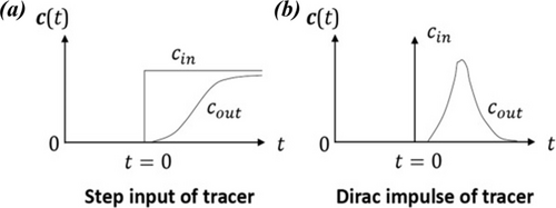
Figure 1. Reactor response to a step input of tracer (a) and to an impulse of a tracer (b) [36].
Bild 1. Reaktion des Reaktors auf eine sprunghafte Zufuhr eines Tracers (a) und auf einen Impuls eines Tracers (b) [36].
where is the time t normalized by the space time τ. The tracer concentration at the inlet of the reactor when n moles of tracer are injected instantaneously in a fluid stream with flowrate Q0 is where δ(t) is the impulse or Dirac delta function, Figure 1b 36.
2.2 Experimental method
2.2.1 Experimental setup
For the experimental studies of the residence time distribution, the company Semperit Technische Produkte GmbH provided a cold-feeding single-screw extruder. The extrusion line consists of a single-screw extruder with two barrel zones (including degassing zone) and a gear pump. The screw has different geometrical configurations along its length and has an outer diameter of 120 mm and the ratio of the length to its diameter (L/D) is 22. The extruder is fed via a feed roller synchronized to the rotational speed of the extruder screw. The rubber compound is fed in form of strips. A single-strip feed was selected for the experimental investigation. To investigate the tracer concentration in the extruded profile cross-section, a tool disc was used to produce a round cord with a diameter of 15 mm.
2.2.2 Material-tracer
The same material in different colours was used for the experiments. This guarantees that there are no additional effects on the throughput behaviour. The material compound is an ethylene propylene diene monomer rubber compound. Before the material compounds were used for the residence time analysis, the two material compounds (red coloured and blue coloured compound) were characterized in the laboratory and the viscosity matched. The viscosity curves of the material compounds were analysed using a rubber process analyser and a high-pressure capillary rheometer.
For the analysis of the colour spectrum in the sample cross-section and a more exact separation between tracer material and carrier material, a calibration curve was determined experimentally. Starting from the basic colours - red and blue - of the material, different mass proportions of red and blue were mixed on a roller mill. The total mass of material to be mixed was kept constant. The colour spectrum of the mixed material masses was evaluated in the same way as the sample images and implemented in the evaluation algorithm.
2.2.3 Experimental procedure
To analyse the residence time behaviour of the extrusion line under consideration, the rotational speed of the extruder screw and temperature difference between the extruder screw and the two barrel zones were changed separately starting from a reference state. The other setting parameters were kept at the value of the reference state. To maintain the pressure at the inlet of the gear pump, the rotational speed of the gear pump was adjusted.
For each parameter variation, the extrusion process was operated until a steady state was reached. Before the tracer strips were fed to the extruder, the strips were weighed to determine the volume of the tracer strip. Then, strips of the tracer material were fed into the extrusion process. The tracer volume is used to validate the detected tracer volume at the end with the amount that was fed into the extruder.
For the determination of the individual output signal curves, samples of the extruded round profile were taken at the outlet of the tool disc. The sampling of the round cord profiles takes place every 20 seconds. In addition to the samples taken, the speed of the extruded profile was measured in each stationary state using a measuring wheel and the shadow dimension was recorded using a laser measuring device to determine the diameter of the round cord profile throughout the experimental testing. The profile samples were deep-frozen to −20 °C and then sample cross-sections were generated for microscopic examination using a mechanical punch.
2.2.4 Modified digital image processing method
To determine the tracer concentration, the samples were placed on a black background and pictures were taken with a Keyence microscope (type: VHX-6000). All images of the sample cross-sections were taken under the same exposure settings of the microscope. In addition, care was taken to maintain consistent environmental conditions. The sample images have a resolution of 1600 x 1200 pixels.
For an automated analysis of the sample images and thus for the generation of the tracer concentration curves, a modified digital image processing method was developed using the digital image processing toolbox of the software MATLAB (version R2021b, Math Works). The development of the method is inspired by a digital image processing method from the field of plasticating extruder 27.
To identify the amount of tracer in the cross-sections of the samples, the tracer colour has to be detected using the colour of each pixel. The colour space hue-saturation-value (detailed information about the hue-saturation-value colour space in the appendix) expresses the perception colour contacts clearer than colour space red-green-blue, so it is adopted widely in the field of image processing 37. Consequently, the stored sample images are converted from the red-green-blue colour space to the hue-saturation-value colour space (value refers to the luminance).
As input, the evaluation algorithm requires the sample images and corresponding time stamps, the calibration curve, as well as the average sample diameter and the velocity of the extruded profile per steady state. After converting the images into the hue-saturation-value colour space, the black background of the samples is removed. The number of pixels of tracer colour was then analysed within the area of the sample cross-section, Figure 2. Thus, using the total number of pixels in the sample cross-section and the number of tracer pixels, the percentage of tracer material in each sample cross-section is determined.
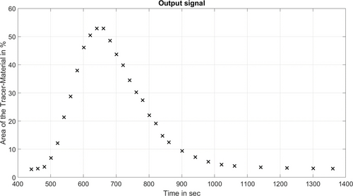
Figure 2. Pixel evaluation of a stationary reference state along the associated product concentration curve.
Bild 2. Pixelauswertung eines stationären Referenzzustandes entlang der zugehörigen Produktkonzentrationskurve.
An example of a typical tracer concentration curve is visualized, Figure 2. The inlay images show the Hue channel of the sample cross-sections.
2.3 Prediction method
The prediction method is separated in two sequences. In the first sequence the identification of the two Gaussian parameters of the extracted residence time distributions are approximated using a curve fitting approach. The data set of the fitted Gaussian parameters is utilized for the training stage of the prediction model. The second sequence are the predictions of the Gaussian parameters within the prediction model at different stationary stage using process parameters, for example the screw speed of the process, as input parameters. The predicted Gaussian parameters enable the regeneration of the residence time distribution of the process.
2.3.1 Parameterizing
For the prediction method, the residence time distribution have to be extracted for each steady state of the experimental studies out of the feed concentration curve and the product concentration curve. The experimental analysis of the impulse response of a linear time invariant system is a common task in diverse areas. For the reason that the system input and output are coupled via the convolution for linear systems, the inverse operation (often known as the filter process) is referred to as deconvolution 38.
To extract the residence time distribution from the experimental data, the assumption is made that the system behaviour in the steady-state operating conditions of the experimental investigations can be replicated to a good approximation as linear time invariant systems. Therefore, a MATLAB (version R20221b, Math Works) internal deconvolution function is used in the developed algorithm for the extraction of the residence time distribution. Before the feed concentration curve and product concentration curve are deconvolved, the two curves are resampled on a common time scale using linear interpolation. An example of the curves is visualized, Figure 3. The product concentration curve has a similar shape to the corresponding residence time distribution, but while the residence time distribution is independent of the system input, the output concentration curve depends on the specific input of the experiment.
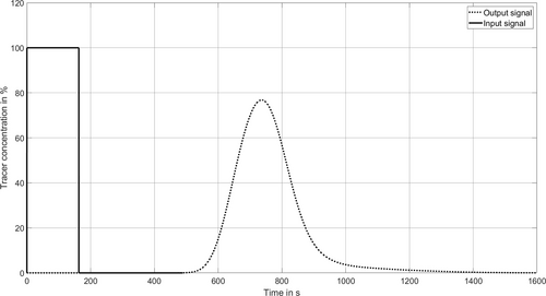
Figure 3. Example of a feed concentration curve and a product concentration curve before deconvolution.
Bild 3. Beispiel einer Zufuhrkonzentrationskurve und einer Produktkonzentrationskurve vor der Dekonvolution.
2.3.2 Prediction
A suitable prediction method was selected based on the available data set and the number of data points. A machine learning method called gradient boosting was chosen. The gradient boosting method is based on the regression method of linear squares boosting. We refer to the literature for a detailed mathematical description of the prediction algorithm used 33, 34.
For the prediction of the residence time distribution out of the data set (Gaussian parameters - expected value μ and the variance σ) depending on the rotational speed of the extruder screw and the tempering of the screw and the two barrels, we use internal functions of the MATLAB Optimization Toolbox. Least squares boosting fits regression ensembles. At every step, the regression ensemble fits a new learner to the difference between the observed response and the aggregated prediction of all previous learners. The ensemble fits to minimize the mean-squared error. To validate the predictions of the residence time distributions, a data set was generated that contains stationary operating states that were not included in the previous experimental investigations.
3 Results and discussion
In order to prove the feasibility of the modified digital image processing method, the reproducibility of the method is investigated. For this purpose, the experiment was repeated under the same conditions. In addition, the material properties were examined in the laboratory in order to exclude deviating material properties in the reference state. Furthermore, the detected tracer volume was calculated and compared with the added volumes of tracer material during the experimental studies. The reproducibility of the method was tested in a pre-defined reference state, Figure 4.
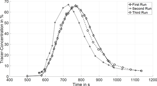
Figure 4. Product concentration curves under the same operating conditions (reference state: screw speed=7.1 min-1).
Bild 4. Produktkonzentrationskurven unter denselben Betriebsbedingungen (Referenzzustand: Schneckendrehzahl=7,1 min-1).
3.1 Experimental method validation
In order to prove the feasibility of the modified digital image processing method, the reproducibility of the method is investigated. For this purpose, the experiment was repeated under the same conditions. In addition, the material properties were examined in the laboratory in order to exclude deviating material properties in the reference state. Furthermore, the detected tracer volume was calculated and compared with the added volumes of tracer material during the experimental studies. The reproducibility of the method was tested in a pre-defined reference state, Figure 4.
A repetition of the analysis of the product concentration curves in the defined reference state was carried out, Figure 4. In the first run, the blue material compound was used as carrier material and the red material compound as tracer material - in the second and third run it was the other way around. The starting point (0 sec) begins when the strip-shaped tracer material is fed into the extrusion process. The product concentration curve reflect the tracer content in the sample cross-section as it exits the extrusion process. The output concentration curves coincide in the reference state, which is an indication of good reproducibility, Figure 4.
The supplied tracer volume - calculated from the weight of the tracer strips and the raw density of the material - was compared with the calculated volume from the concentration curves. For the experimental product concentration curves, the total tracer material could be detected at the outlet of the extrusion process with a maximum deviation of less than 6 % using the digital image processing method, Figure 4.
3.2 Effect of parameter variations
According to the findings of the existing literature, the focus of the experimental investigations was placed on the influences of variations in the screw speed and the temperature of the screws and the two barrels on the throughput behaviour of the extrusion process. The variation of the screw speed were visualized to analyse the influence on the throughput behaviour respectively on the residence time distribution of the extrusion process, Figure 5. The gear pump speed was adjusted to maintain constant pressure at the inlet of the gear pump and to avoid undesirable influences on the flow in the screw channel.
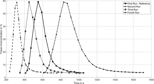
Figure 5. Variation of the rotational speed of the extruder screw (reference state: 10.3 min-1; second run: 18.9 min-1; third run: 12.9 min-1; fourth run: 6.6 min-1).
Bild 5. Variation der Drehzahl der Extruderschnecke (Referenzzustand: 10,3 min-1; zweiter Lauf: 18,9 min-1; dritter Lauf: 12,9 min-1; vierter Lauf: 6,6 min-1).
At a higher screw speed (second and third run), a shift of the concentration curve towards shorter throughput times can be observed. In addition, the curve becomes sharper as the screw speed increases. The opposite effects can be observed at reduced screw speeds. The effects of the variation in tempering were also visualized, Figure 6. With an increased screw temperature and a reduced barrel temperature, the concentration curve shifts to earlier times. However, the effect of the tempering is not as pronounced as with the variations in screw speed. An opposite effect can be recognized when the barrel temperature is increased and the screw temperature is reduced at the same time.
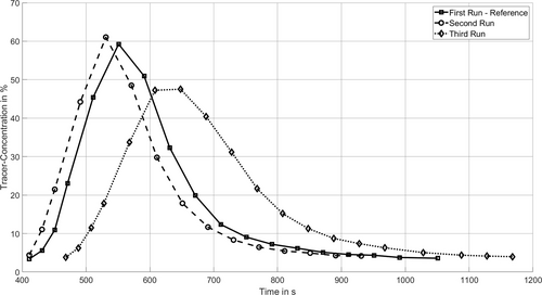
Figure 6. Variation of the tempering of screw and the two barrels (reference state: screw=70 °C, barrel 1=70 °C, barrel 2=50 °C; second run: screw=90 °C, barrels=50 °C; third run: screw=50 °C, barrels=90 °C).
Bild 6. Variation der Temperierung der Schnecke und der beiden Zylinder (Referenzzustand: Schnecke=70 °C, Zylinder 1=70 °C, Zylinder 2=50 °C; Zweiter Lauf: Schnecke=90 °C, Zylinder=50 °C; Dritter Lauf: Schnecke=50 °C, Zylinder=90 °C).
The throughput behaviour was also analysed using the experimentally determined volume flow. Our results are qualitatively in accordance with the findings of previous studies 1, 2, 27.
3.3 Parameterizing
As already described in the methods section, the residence time distributions - corresponding to the transfer function in the respective stationary operating state - are extracted from the experimentally recorded feed concentration curves and the product concentration curves using the mathematical operation of deconvolution. An example of a deconvoluted residence time distribution including the Gaussian fit is illustrated, Figure 7. In order to create a suitable data set for predicting the residence time distribution of the process, the Gaussian coefficients - expected value μ and variance σ - were extracted for 30 different steady-state operating conditions. The mean value of the coefficient of determination R2 for all operating states is 0.96.
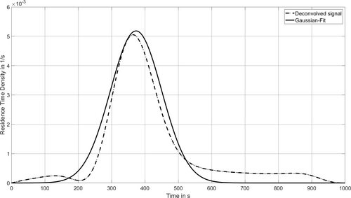
Figure 7. Deconvoluted residence time distribution (transfer function) and the result of the Gaussian fit.
Bild 7. Dekonvolutierte Verweilzeitverteilung (Übertragungsfunktion) und Ergebnis der Gauß-Anpassung.
When analysing the experimental data, it was discovered that the spread of the data for the tempering was insufficient. For this reason, a data analysis of the experimentally determined volume flow was executed, which also reflects the effects in the throughput behaviour in the case of a change in tempering. If the screw tempering is increased and the tempering of the barrels are reduced at the same time, the product concentration curve is shifted to earlier times. These changes in tempering also cause an increase in the prevailing volume flow. If the screw tempering is reduced and the tempering of the barrels are increased at the same time, the opposite occurs. Therefore, the volume flow rate was selected as a second independent parameter alongside the screw speed in order to include the influence of tempering on the residence time distribution in the predictions. As the volume flow also correlates with the screw speed, the correlation between screw speed and volume flow was resolved by normalizing the volume flow within the screw speed in advance. The results of the parameterization of the residence time distributions from the experimental training data including (blue dots) the validation data (red diamonds) are shown, Figures 8, 9.
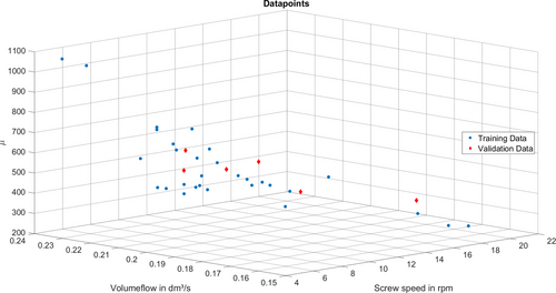
Figure 8. Results of the Gaussian fit for the expected value μ.
Bild 8. Ergebnisse der Gauß-Anpassung für den erwarteten Wert μ.
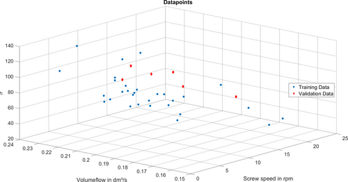
Figure 9. Results of the Gaussian fit for the variance σ.
Bild 9. Ergebnisse der Gauß-Anpassung für die Varianz σ.
3.4 Predictions
The results regarding the prediction of the residence time distribution of the extrusion process using the two Gaussian coefficients extracted from the deconvoluted residence time distributions are presented and discussed in this section. Additional experimental data was generated to validate the prediction accuracy of the developed method. The extracted Gaussian coefficients of the validation data have already been introduced, Figures 8, 9. For the generation of the validation data, both steady-state operating conditions within the data space of the existing data and steady-state operating conditions outside the existing data space were tested. The data space of the training data set ranges from approximately 7 min−1 to 19 min−1 for the screw speed and from approximately 50 °C to 90 °C for the tempering zones. For the validation of the prediction method, the residence time distributions of six steady states were deconvoluted and the Gaussian coefficients were extracted. Three of the six states - center right, bottom left and bottom right - are outside of the space of the training data, Figure 10.
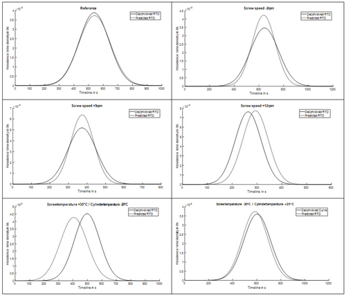
Figure 10. Comparison of the predicted residence time distributions with the deconvolved residence time distributions of the validation data (reference state: screw=10 min-1, screw temperature=70 °C, barrel 1=70 °C, barrel 2=50 °C; top right: screw=8 min-1, tempering zones=reference state; center left: screw=15 min-1, tempering zones=reference state; center right: screw=22 min-1, tempering zones=reference state; bottom left: screw=reference state, screw temperature=50 °C, barrels=95 °C; bottom right: screw=reference state, screw temperature=100 °C, barrels=50 °C).
Bild 10. Vergleich der vorhergesagten Verweilzeitverteilungsdichten mit den dekonvolvierten Verweilzeitverteilungsdichten der Validierungsdaten (Referenzzustand: Schnecke=10 min-1, Schneckentemperatur=70 °C, Zylinder 1=70 °C, Zylinder 2=50 °C; Oben rechts: Schnecke=8 min-1, Temperierungszonen=Referenzzustand; Mitte links: Schnecke=15 min-1, Temperierungszonen=Referenzzustand; Mitte rechts: Schnecke=22 min-1, Temperierungszonen=Referenzzustand; Unten links: Schnecke=Referenzzustand, Schneckentemperatur=50 °C, Zylinder=95 °C; Unten rechts: Schnecke=Referenzzustand, Schneckentemperatur=100 °C, Zylinder=50 °C).
The prediction of the expected value σ within the data space of the training data is a sufficiently accurate prediction, Figure 10. Outside the training data set, the prediction accuracy for the variance μ of the residence time distributions is more accurate. An overview of the results regarding the validation of the prediction method in the form of the absolute deviations in percent for the two Gaussian coefficients was carried out, Table 1.
Steady state |
Relative deviation of expected value μ in % |
Relative deviation of variance σ in % |
|---|---|---|
Reference state |
2.77 |
0.77 |
Screw speed=22 min-1 |
1.44 |
11.13 |
Screw speed=15 min-1 |
18.7 |
0.2 |
Screw speed=8 min-1 |
18 |
1.01 |
Screw temperature=100 °C, Barrels=50 °C |
5.99 |
18.51 |
Screw temperature=50 °C, Barrels=95 °C |
3.73 |
2.94 |
4 Concluions and outlook
In the present work, we showed an experimental procedure to detect and analyse the residence time distribution using a digital image processing method. The results of the experimental investigations indicated a good reproducibility. In addition, the method was used to analyse the effects of different screw speeds and different tempering of the screw and the two barrels on the residence time distribution of the extrusion process. Research is underway to use the described method for analysing the effects of different process variables (e. g. material parameters) on the residence time distribution of the rubber extrusion process. It should also be emphasized that the time required to generate the experimental data is considerable. However, in industrial extrusion processes, it is commonly the case that the products to be produced are manufactured with the same starting material or that a large quantity of the same product is extruded and thus the developed method is a promising application possibility.
Furthermore, we presented a mathematical method how the residence time distribution (corresponding to the transfer function) can be deconvoluted from experimental data respectively from input and output signals. The subsequent curve fits of the residence time distributions (Gaussian fit) could be performed with sufficient accuracy - R2 around 0.96 for all 30 training data points. The deviation of the prediction method using the machine learning method named gradient boosting could be predicted for the Gaussian coefficients - expected value μ and variance σ - with a deviation of less than 6 % and less than 9 % respectively. In the course of further research activities, the experimental investigations and the parameter range of the stationary states of the process are to be expanded in order to achieve a higher prediction accuracy.
To summarize, we have developed a promising prediction method for the residence time distribution of the rubber extrusion process. Since the production limits of the process strongly depend on the residence time distribution and modern control approaches (e. g. model predictive control) require the information in a sufficiently short computing time, the presented method is a promising approach even if it is based on some simplifications. The use of modern control techniques coupled with more accurate prediction of processing limits could help transform the rubber extrusion process into a more efficient and resource-saving mode of operation.
Acknowledgements
The authors express their gratitude to Semperit Technische Produkte GmbH for the provision of the extrusion line and the laboratory equipment for the experimental investigations. The authors acknowledge funding support of this work through the research project DigiTEx (FFG project number 907976). The authors acknowledge TU Wien Bibliothek for financial support through its Open Access Funding Programme.
Conflict of Interests
The authors declare no financial or commercial conflict of interests.
Open Research
Data Availability Statement
Data sharing not applicable due to confidentiality agreements.


