We present ichor, an open-source Python library that simplifies data management in computational chemistry and streamlines machine learning force field development. Ichor implements many easily extensible file management tools, in addition to a lazy file reading system, allowing efficient management of hundreds of thousands of computational chemistry files. Data from calculations can be readily stored into databases for easy sharing and post-processing. Raw data can be directly processed by ichor to create machine learning-ready datasets. In addition to powerful data-related capabilities, ichor provides interfaces to popular workload management software employed by High Performance Computing clusters, making for effortless submission of thousands of separate calculations with only a single line of Python code. Furthermore, a simple-to-use command line interface has been implemented through a series of menu systems to further increase accessibility and efficiency of common important ichor tasks. Finally, ichor implements general tools for visualization and analysis of datasets and tools for measuring machine-learning model quality both on test set data and in simulations. With the current functionalities, ichor can serve as an end-to-end data procurement, data management, and analysis solution for machine-learning force-field development.

1 INTRODUCTION

Computational chemistry continues to evolve both theoretically and computationally.^1-3 Today, computational chemistry has become paramount as it is highly integrated with areas such as drug discovery,^4-10 materials science,^11-16 catalysis,^17-26 and environmental chemistry.^{27, 28} Computational chemistry algorithms are implemented in multiple off-the-shelf computer programs, which are available either freely or commercially. However, at the moment, the ability to quickly switch between programs is limited due to drastically different file formats between programs, even if the programs themselves perform similar functions.

Although concerns have been voiced over the development process of computational chemistry software and the necessity to build standards and increase interoperability,^29-31 it is highly unlikely that similar computational chemistry software will adopt identical file formatting standards in the foreseeable future. This is due to a variety of reasons, such as time constraints, reliance on legacy code, competitiveness, and the closed-source development process of most computational chemistry programs. Therefore, at present, the only straightforward way to automate computational chemistry workflows is to write additional code, which then interfaces with the relevant programs used in the workflows.

There are multiple libraries that already address issues relating to computational chemistry file reading and writing, such as cclib,³² IOData,³³ pymatgen³⁴ and Open Babel.³⁵ These libraries are perfectly suitable for file reading and writing tasks but more tools are required for cases where thousands of files from multiple separate calculations (and multiple software programs) need to be handled. More automation for computational chemistry file management is possible, and would bring several benefits to the end user, such as faster data processing times, improved data organization and accessibility, and better interoperability, with the latter two being key objectives of the FAIR Data Principles.³⁶ Automation will also increase reproducibility of results, as well as streamline data curation and processing, which is critical for use cases such as machine learning (ML).

ML datasets collate results from hundreds of thousands of separate calculations. Therefore, a large amount of compute resources, in terms of both high processing power and throughput, are required for ML dataset construction. The calculations are most often performed on large centralized High-Performance Computing (HPC) or High-Throughput Computing (HTC) clusters that drastically improve access to both hardware and software. Workload managers such as Sun Grid Engine (SGE) and SLURM are software tools commonly installed on the clusters to schedule and manage user calculations (called jobs). Multiple jobs can be submitted by different users at once and the workload management software on the cluster ensures the appropriate compute resources are allocated.

Workload managers are necessary but they add an extra layer of complexity that compute cluster users must be knowledgeable about. Additionally, compute clusters are dominantly Linux-based, such that users must also be familiar with basic Linux commands and operations prior to utilizing the cluster. Although there is a wide amount of readily available documentation on both Linux and the workflow managers, the substantial background knowledge required to submit calculations still poses a barrier to entry, especially to inexperienced researchers. Fortunately, further automation relating to workload managers job submission is possible and allows for seamless switching between compute clusters, while also removing the need for manual job creation and submission, which can itself be time consuming.

As the demand for in silico modeling continues to increase in the future, there is a concomitant need for further automation in computational chemistry workflows. There are already packages such as the atomic simulation environment (ASE),³⁷ atomate³⁸ (previously FireWorks³⁹), and PLAMS,⁴⁰ which have gained popularity in recent years and address various parts of computational chemistry workflows. These packages have proven to be highly sought-after research tools because they decrease the chance of errors and increase reproducibility of calculations, all while simplifying how computational research is conducted.

Finally, the recent increase in popularity of ML and its use for so-called ML force fields (FFs), has increased the need for high-volume processing of datasets. While there is a plethora of proposed ML frameworks, currently tools for dataset processing are scarce,^41-43 and packages for analysis of ML FF models (and resulting simulations) have not been widely discussed. Standardized testing of ML model performance, both in terms of prediction accuracy and simulation stability, will allow for much more straightforward comparison of different models. There is already emerging literature discussing the need for more thorough benchmarking for ML FFs.⁴⁴

In this work, we present ichor, a fully open-source Python package for computational chemistry data management and machine learning force field development. Ichor can interface with any computational chemistry software, automate HPC and HTC-related workflows, as well as manage and process any input and output data from calculations. Starting as a project to improve the in-house GAIA^{45, 46} pipeline, the code was developed particularly for the use in ML FF development, with the goal of being an all-in-one solution for dataset construction and ML model analysis that is easy to use and to extend. Although the primary intent for ichor is to aid ML FF development, the parts of ichor that deal with job submission and data collection are general enough to find uses in many other computational chemistry areas. Tasks relating to job submission and data collection are very similar across research domains, so in practice the ichor code can also manage non-computational chemistry related data. The main goals of ichor are to:

Provide an easy-to-use interface to any computational chemistry software in order to improve efficiency and allow seamless switching between similar software.
Define and implement flexible data structures to allow for effortless data access from any number of calculations performed by multiple different programs.
Integrate common database formats for long-term data storage to allow for efficient post-processing and sharing of data.
Provide interfaces to compute cluster management software, thereby removing the need to manually write submission scripts, making workflows portable between clusters.
Collate tools relating to ML dataset and model analysis, as well as simulation performance benchmarking.

Ichor is a Python namespace package that unites three individual packages: ichor.core, ichor.hpc and ichor.cli. The ichor.core package implements file parsing, data structures, databases, data post-processing functionalities, as well as tools for analysis of ML models and simulations. The ichor.hpc package contains interfaces for workload managers and automates job script construction and submission. The high-level Python code, which is used by the end user, is agnostic to the workload manager that is installed on the compute cluster. Finally, ichor.cli provides a very intuitive command line interface (CLI) menu system, which gathers commonly used ichor functionality into one place. The intent of the CLI is to further simplify and speed up tasks and allow even inexperienced ichor users to perform calculations with ease. An overview of a previous ichor version, which was focused on the ML-related aspects of ichor, can be found in a previous publication.⁴⁷ In contrast, after many upgrades of ichor since that publication, the current work focuses on the data management and data processing capabilities of ichor conveying many more details.

2 DATA MANAGEMENT

The ichor.core package implements many data management functionalities including file reading and writing, data structures for managing many input and output files, as well as long-term database storage of important results. Setting up input files for calculations as well as extracting data from said calculations is a very common task in computational chemistry, which can and should be automated. While manual modification and management is possible when dealing with only a few jobs, it becomes impractical and inefficient when dealing with many calculations at once. As ML datasets for FF development rely on data generated from thousands of separate calculations, data management becomes a critical component of the ML pipeline. Efficient data management can only be carried out by establishing a structure, both on disk and in code, which gathers similar calculations and allows for quick data access from hundreds of thousands of calculations. Currently, the ichor code is interfaced with AMBER,⁴⁸ CP2K,⁴⁹ GAUSSIAN,⁵⁰ ORCA,⁵¹ TYCHE,⁵² DL_POLY⁵³ and AIMAll.⁵⁴

2.1 File reading and writing

Ichor implements abstractions for file reading and writing, which can easily accommodate any new file formats. There are two main abstract base classes, ReadFile and WriteFile , which are subclassed by file-related classes that read and/or writes files, respectively. To improve the efficiency of file parsing, a lazy file reading system has been developed, which only reads files when necessary. Important results from files, such as the total system energy from GAUSSIAN or ORCA calculations, are cached after initially reading the files. It is very straightforward to modify existing ichor code and add new data to the cache. Lazy file reading is critical in cases where information is only needed from a fraction of the full set of files, saving valuable time. In addition, accessing data lazily allows for implementation of efficient high-level data structures, which can be used to collectively obtain information from hundreds of thousands of files. Lazy file reading is inherited by all subclasses of the ReadFile class. Ichor implements both file reading and writing for computational chemistry program input files. For output files, it is usually only necessary to implement file reading methods because output files are created by the relevant software that performs the calculations.

The ichor code is designed to be as easy to use as possible, where a single Python class handles all three scenarios of the state of a particular type of file: (i) the file is already present on disk and requires no further modifications, (ii) the file is present on disk but modifications to the contents of the file are needed, or (iii) the file is not present on disk and needs to be constructed from scratch and subsequently written to disk. In the first scenario, the input file can be read directly by ichor or used as input to the respective computational chemistry program. In the second scenario, ichor can be used to modify the contents of the file, and any specified changes can be written to the file on disk. In the third and final case, the user can build files from scratch directly through the ichor code. Any required parameters, such as the chemical structure, must be provided by the user but optional calculation parameters are filled with sensible defaults. For example, the user must provide the starting geometry for an electronic structure calculation, but a default basis set and method are set by ichor. Of course, the user has the ability to change any settings if the default ones are not suitable.

Below is an example of using ichor to manage GAUSSIAN and ORCA input files. Both of these programs are used for electronic structure calculations and require identical input information, such as the molecular configuration and level of theory. Using ichor, it is straightforward to construct and interchange input file formats like so:

>>> from ichor.core.files import XYZ, GJF, OrcaInput

>>> atoms = XYZ("methanol.xyz").atoms # get molecular configuration

>>> gjf = GJF("gaussian_input.gjf", basis_set="aug-cc-pvtz")

>>> gjf.atoms = atoms

>>> gjf.write() # writes file to disk

>>> orca = OrcaInput("orca_input.orca", method="bp86")

>>> orca.atoms = atoms

>>> orca.write()

The XYZ class is used for convenience to obtain a chemical structure but in practice a chemical structure can be defined directly by using the ichor Atoms class. Instances of the GJF , and OrcaInput classes are created, and the “atoms” attribute is assigned to the Atoms instance from the “xyz” input file. As an example, the aug-cc-pVTZ basis set is used for the GAUSSIAN input file. The new files are then written to disk using the write method. The contents of the files that are written, as well as the example methanol geometry, can be found in Sections 1–3 of the Supplementary Information (SI). The contents of the files can be modified with the exact same classes as follows:

>>> orca_input = OrcaInput("orca_input.orca", basis_set="aug-cc-pvdz")

>>> orca_input.basis_set # instance is modified, but changes not written to file yet.

'aug-cc-pvdz'

>>> orca_input.write() # modifications now written to file

Once the files are written to disk, the exact same classes as before can be used to read from disk the contents of the files. Reading in the files that were written out in the previous step yields the following example results:

>>> gjf = GJF("gaussian_input.gjf")

>>> orca = OrcaInput("orca_input.orca")

>>> gjf.basis_set

'aug-cc-pvtz'

>>> orca.method

'bp86'

In addition to a write method to write files, ichor does implement a read method to read files. However, as seen in the code snippet above, there is no need to explicitly call the read method in order to read the contents of the file, which is a result of the lazy file reading system. Instead, by lazy evaluation,⁵⁵ the contents of the file are read only when attributes of the instance are accessed. Once the contents of the file are read for the first time, attributes of the corresponding instance are populated with the data contained in the file. Omitting the need for calling the read method seems like a small implementation detail, but it has completely removed the potential for workflow bugs caused by forgetting to explicity call the read method and has allowed for dynamic reading of files.

The ichor file handling code can be used in combination with any of the powerful computational chemistry file parsers that are already implemented in other Python libraries. Therefore, new file formats supported by other libraries can be readily added into ichor without the need to reinvent the wheel and write additional file parsing code. Benefits of the ichor code base, such as lazy file reading and higher-level data management functionalities, are still present, even if the parsing implementations are outsourced to another library. Additionally, ichor file classes can abstract away implementation details of third-party libraries and define a uniform interface to read, modify, and write any type of file. Examples of interfacing ichor with third-party libraries for file parsing can be found in the ichor documentation (see Data Availability section).

2.2 High-level data structures

When dealing with thousands of separate calculations, as in the case of ML FF datasets, it becomes necessary to define data structures to simplify setting up and running calculations, as well as to manage input and output data. The data structures in ichor are implemented in a bottom-up approach, where methods to access relevant data are written for the classes that handle individual files. Subsequently, these methods are utilized by higher-level classes that pool data from multiple different files. The high-level data structure code is written in a highly modular fashion, allowing the end user to easily swap between different input and output files from any of the supported computational chemistry programs. For our ML pipeline we have developed the data structures seen in Figure 1.

Details are in the caption following the image — **FIGURE 1**
Open in figure viewer PowerPoint

Modular data structures in the ichor package. The objects in orange are Python classes that are used to handle data from individual files or sub-directories. The **PointDirectory** object encapsulates all data for a single system configuration (a point). The **PointsDirectory** object contains multiple **PointDirectory** objects and can be used to efficiently obtain data from all calculations. Finally, the **PointsDirectory** instance can be converted to a database for long-term storage.

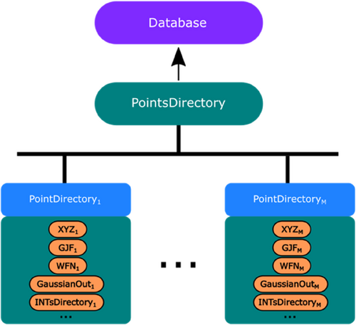
The lowest data structure layer contains classes for managing individual files (e.g., the GJF Python class is used to parse GAUSSIAN “gjf” input files) or individual sub-directories (e.g., the IntsDirectory class is used to gather data from multiple Int instances, which themselves contain atomic integration results from “int” files produced by the quantum topological program AIMAll). All data obtained from individual Int instances is readily accessed through IntsDirectory . There are many other file handling Python classes, such as WFN , and GaussianOut , which handle “wfn” (wavefunction) files and GAUSSIAN output files respectively.

Because multiple programs can be chained in sequence, where the output data from one program is fed into another program, it becomes highly beneficial to bundle all calculations relating to one molecular structure. The PointDirectory class is used to contain all information for a single system configuration (i.e., a point). This Python class encapsulates a single directory containing any number of files or sub-directories, which in turn contain all the information for the particular geometry (which is stored in the “xyz” file). For a dataset consisting of $M$ points, there are going to be $M$ directories created on disk, and therefore $M$ instances of the PointDirectory class will be necessary.

An example PointDirectory -like directory structure containing information from GAUSSIAN and AIMAll can be seen in Figure 2A, while Figure 2B contains data from ORCA and AIMAll instead. Either of the electronic structure codes can be used to produce a “wfn” file, which contains the molecular orbital coefficients. The AIMAll program then uses the “wfn” file to calculate properties associated with topological atoms, such as the Interacting Quantum Atoms (IQA)⁵⁶ energy and atomic multipole moments.

Using PointDirectory , a user can very easily access all relevant contents from files or sub-directories contained inside. Below is an example of accessing the total energy and virial ratio from the wavefunction file “WM0000.wfn” from Figure 2A, as well as the Cartesian forces and molecular multipole moments from the GAUSSIAN output file:

>>> from ichor.core.files import PointDirectory

>>> pd = PointDirectory("WM0000.pointdir")

>>> pd.wfn.raw_data

{'energy': ‐76.399967044227, 'virial_ratio': 2.00535371}

>>> pd.gaussian_output.raw_data

{'global_forces': {'O1': array([‐0.27867968, ‐0.00110596, 0. ]), 'H2': array([ 0.24439694, 0.02135532, ‐0. ]), 'H3': array([ 0.03428274, ‐0.02024935, ‐0. ])}, 'charge': 0, 'multiplicity': 1, 'molecular_dipole': MolecularDipole(x=0.6742, y=1.716, z=‐0.0), 'molecular_quadrupole': MolecularQuadrupole(xx=‐4.6534, yy=‐5.7932, zz=‐7.7592, xy=‐1.329, xz=0.0, yz=‐0.0), 'traceless_molecular_quadrupole': TracelessMolecularQuadrupole(xx=1.4152, yy=0.2754, zz=‐1.6906, xy=‐1.329, xz=0.0, yz=‐0.0), 'molecular_octapole': MolecularOctapole(xxx=0.7933, yyy=0.2957, zzz=‐0.0, xyy=‐0.788, xxy=0.2469, xxz=‐0.0, xzz=0.0233, yzz=‐0.2965, yyz=‐0.0, xyz=0.0), 'molecular_hexadecapole': MolecularHexadecapole(xxxx=‐5.9359, yyyy=‐7.1655, zzzz=‐7.8237, xxxy=‐0.2656, xxxz=0.0, yyyx=‐0.6628, yyyz=‐0.0, zzzx=0.0, zzzy=0.0, xxyy=‐2.0681, xxzz=‐2.5253, yyzz=‐2.6926, xxyz=‐0.0, yyxz=0.0, zzxy=0.0417)}

Using PointDirectory , all relevant data contained in all sub-files or directories can be accessed in the following way:

>>> from ichor.core.files import PointDirectory

>>> pd = PointDirectory("WM0000.pointdir")

>>> pd.raw_data

{'gaussian_output': … , 'wfn': …, 'ints': …}

where ellipses have been used to truncate all the information to save space. Essentially, the code snippet above parses all files that contain calculation data and returns a Python dictionary with all the parsed information. The full output of this command can be found in Section 4 of the SI.

It is very important to note that the contents of a PointDirectory can be switched quickly in the case that new computational chemistry programs are used for calculations. To change the content types, the contents class variable of PointDirectory can be overridden. This capability allows for very easy customization of PointDirectory depending on the types of files that are present in the directory. For example, if ORCA is used for the electronic structure calculations, then the file contents contained in the PointDirectory object are going to be substantially different, as seen in Figure 2B. Through ichor it is trivial to parse the contents from another computational chemistry program like so.

>>> from ichor.core.files import OrcaInput, OrcaOutput, OrcaEngrad, PointDirectory

>>> PointDirectory .contents = {"input": OrcaInput, "output": OrcaOutput, "engrad", : OrcaEngrad}

>>> pd = PointDirectory ("WM_ORCA0000.pointdir")

>>> pd.engrad.raw_data.

{'global_forces': {'O1': array([‐7.11005321e‐03, 6.46768420e‐02, ‐3.70300000e‐09]), 'H2': array([‐3.29989815e‐03, ‐2.91027685e‐03, 1.34300000e‐09]), 'H3': array([ 1.03813014e‐02, ‐6.18227788e‐02, ‐2.06000000e‐10])}, 'total_energy': ‐76.427541336208}

The keys of the contents dictionary are automatically accessible as attributes of the PointDirectory instance. Any of the implemented File or Directory -like classes can be passed into the contents dictionary, ensuring that customized file types and file structures can be built efficiently and effortlessly. These data structures allow for easy comparison of results between different programs, without the need to do any manual file manipulation. The ability to readily switch between computational chemistry programs has several benefits: (i) performing benchmarks to find the optimal program (and settings) for the task at hand, (ii) accessing complementary feature sets of multiple different programs, as well as (iii) allowing direct comparison of results obtained by similar software, which leads to (iv) aiding with finding implementation differences between programs. The PointDirectory class implemented in ichor serves as a template from which further customization of data structures can follow.

Previous examples showed how to obtain raw data from calculations, however most of time, some post processing or analysis of the raw data is required. Post-processing of information in a PointDirectory is very simple to do by writing a Python function that processed the contents of a PointDirectory instance. For example, a simple processing function can be written which compares the GAUSSIAN system energy

(E_{Gaussian})

to the sum of atomic energies

(E_{IQA}^{A})

calculated by AIMAll. The absolute error (in kJ mol⁻¹) is defined in Equation (1),

error = |E_{Gaussian} - \sum_{A} E_{IQA}^{A}|,

(1)

The above equation can be translated into code and applied to a PointDirectory as follows:

>>> def energy_diff(point_dir: PointDirectory):

>>> …. iqa_sum = sum([i.iqa for i in point_dir.ints])

>>> …. total_energy = point_dir.wfn.total_energy

>>> …. return 2625.5 * abs (iqa_sum - total_energy) # convert to kJ mol-1

>>> pd.processed_data(energy_diff)

0.01815745386915779

where 2625.5 is used as a conversion from Hartree to kJ mol⁻¹. The above example is trivial but the procedure for building more complicated PointDirectory processing functions remains exactly the same. Since the raw data are trivial to obtain through the high-level functionality in ichor, post-processing of data also becomes simpler to do.

The PointsDirectory class encapsulates information from multiple PointDirectory -like directories at once. Data for all or a subset of PointDirectory instances contained inside can be accessed through PointsDirectory , essentially meaning this class encompasses a ML dataset with data from thousands of calculations for various system configurations.

For example, the raw data for the whole dataset can be readily accessed by:

>>> pointsdir = PointsDirectory("WM.pointsdir")

>>> pointsdir.raw_data

{'WM0000': {'gaussian_output': … , 'wfn': …, 'ints': …}, 'WM0001': {'gaussian_output': … , 'wfn': …, 'ints': …}, … }

The raw data for all points contained inside the PointsDirectory is returned as a Python dictionary, containing the names of the PointDirectory instances as the keys and the raw data associated with each PointDirectory instance as the values. Note that the output has been truncated and information for only two points is shown. For real datasets there are going to be thousands of points, each containing their own set of data. The full output of the command for the first two points can be found in Section 5 the SI.

2.3 Construction of machine learning databases

Accessing raw data from a large number of files becomes costly because more time is spent parsing files to extract important information. This activity drastically slows down further data processing and makes sharing of ML datasets more difficult. To make data more accessible, databases must be used to store the large amount of data from calculations. Only relevant data are stored in the databases, which drastically reduces the file size of the databases when compared to the original files, leading to easier and faster sharing of data with others. Additionally, databases can be readily queried and filtered by different criteria, which is a very powerful tool for data analysis.

The PointsDirectory class discussed in the previous section provides ways to store relevant data from computational chemistry calculations into databases. Initially, data must be read from the input and output files and collected in the database. However, once this process is completed once, all relevant data can be obtained directly from the database at much faster speeds, eliminating the need for the slow file parsing. The high-level PointsDirectory class can readily be converted into an SQLite3 and JSON formats like so:

>>> pointsdir = PointDirectory ("WM.pointsdir")

>>> pointsdir.write_to_sqlite3_database()

>>> pointsdir.write_to_json_database()

Both databases were specifically designed for storing atomic and molecular property data that are relevant for ML FF development. In particular, data such as atomic coordinates and types, total system energy, forces exerted on the atoms, as well as atomic energies and multipole moments are stored. A schema of the current SQLite3 database format, as well as a truncated example of the JSON database format, can be found in Sections 6 and 7 in the SI. Although it is possible to modify the tables inside this SQL database to accommodate for new types of results, it requires significant prerequisite knowledge of databases and it is time consuming. On the other hand, the JSON database format is much more flexible in terms of types of data that can be stored. The current JSON database implementation can be easily modified to accommodate any new data that may be needed for further processing.

It must be noted that the SQL-based database inherently provides very useful SQL-querying capabilities that are not present in the JSON format by default. However, it is trivial to load in the JSON database and carry out further data filtering in a Python script. Support for other storage formats, such as NoSQL, is planned for future ichor releases. NoSQL combines benefits of SQL and JSON, allowing efficient querying while supporting more data types than SQL. Much like the JSON database format, the NoSQL storage format would also allow users to design and create their own database formats to suit their needs.

3 AUTOMATING WORKLOAD MANAGER JOBS

Computational chemistry tasks are often submitted on HPC or HTC clusters because calculations are resource-intensive and because common computational chemistry software is already installed on clusters. In most cases, it is up to the user to write out job scripts, which define job parameters, such as the number of CPU cores. These parameters are subsequently passed onto the workload manager and then the computational chemistry program. Different HPC clusters may use different workload management software, which hinders the ability to move workflows across clusters. Since job scripts are typically not interchangeable between different workload managers, job scripts need to be modified before jobs can be submitted on other clusters, which utilize different workload managers.

Without automation, the user must be very familiar with the job submission system deployed on the compute cluster. This presents an inconvenience, especially when submitting jobs on multiple clusters with different workload managers. To automate the job submission process, the ichor.hpc package provides interfaces to modern HPC or HTC workload managers, allowing users to submit jobs without knowing the workload manager details on each cluster and reuse the same code across clusters. Users may seamlessly move workflows between clusters without spending time manipulating job scripts, which drastically increases efficiency. In short, ichor aims to abstract away the technicalities associated with each individual workload manager. At the moment, the SGE and SLURM workload managers are supported but other job management software can be readily implemented in the existing ichor code.

3.1 Job submission

A basic example of submitting GAUSSIAN jobs through ichor is this:

>>> from ichor.hpc.submission_script import SubmissionScript

>>> from ichor.hpc.submission_commands import GaussianCommand

>>> files_to_submit = ["file1.gjf", "file2.gjf"]

>>> with SubmissionScript ("submit.sh", ncores=2) as submission_script:

>>> …. for f in files_to_submit:

>>> …. …. submission_script.add_command(GaussianCommand(f))

>>> …. submission_script.submit()

The SubmissionScript class is used to write out submission script files (commonly shell “sh” files), which contain the parameters of the job. This class automatically formats settings to work with the workload manager that is installed on the compute cluster. Parameters such as number of cores to allocate to the job (or array tasks), the locations of standard output and error, special node requests, etc. can be specified though the SubmissionScript Python class. Once the submission script is defined, commands to be submitted on compute nodes are added to the SubmissionScript instance. For example, if GAUSSIAN calculations are to be submitted, the GaussianCommand class is added to the submission script. The command-type classes contain the paths to program executables, as well as the input and output file paths that the program will make use of. Once all jobs are added to the submission script, the script is submitted to the workload manager, which then allocates the specified computational resources. When multiple identical commands are added to a job script, they are automatically converted into an array job.

There are several convenience functions that are already available, allowing one to submit array jobs, each containing thousands of tasks, with just one line of Python code. These functions drastically automate the machine learning dataset building process. For example, one can easily submit thousands of calculations by the following code snippets:

>>> from ichor.hpc.main import submit_points_directory_to_gaussian

>>> submit_points_directory_to_gaussian("WM.pointsdir", basis_set="aug-cc-pvtz")

>>> from ichor.hpc.main import submit_points_directory_to_orca

>>> submit_points_directory_to_orca("WM.pointsdir", main_input=["verytightscf"])

The code snippets above directly submit a PointsDirectory -like directory, containing thousands of different configurations, to either GAUSSIAN or ORCA. These submit-functions handle input file creation, job script creation, as well as job script submission to the workload manager. Log files are created when submitting jobs, allowing one to easily see which jobs were submitted in the past, as well as troubleshoot problems with job submission. Keyword arguments containing additional calculation settings can be specified and will be written to the relevant input files. The user has full control over all calculation settings, allowing submission of advanced job scripts and calculations through just a single line of Python code.

3.2 Ichor configuration file

It is expected that compute clusters are set up differently, therefore utilities such as locations of program executables, will differ across clusters. Ichor uses a yaml-formatted configuration file, “ichor_config.yaml”, to store specific compute cluster details thereby ensuring the portability of the ichor code to any computing environment. Currently, the configuration file should be placed in the home directory of the user. The general structure of the configuration file is:

csf3:

parallel_environment:

smp.pe: [2, 32].

software:

gaussian:

executable_path: "$g09root/g09/g09"

modules: ["/apps/gaussian09"]

cp2k:

executable_path: "cp2k.ssmp"

modules: ["/apps/cp2k/6.0.1"]

data_path: "/opt/apps/cp2k/6.0.1/data"

The top-level key contains the name of the cluster, which should be found when running hostname on the Linux terminal or using similar commands from Python. The parallel_environment key stores information relating to core counts and settings used by the cluster and workload manager. The software key contains settings for programs, such as executable paths, modules that need to be loaded to gain access to software, and additional program-specific configuration settings. The configuration file can contain instructions for multiple clusters at once. As more functionality is added to the code base, the exact structure of the configuration file will likely change. Therefore it is recommended to look at the ichor documentation for the most up-to-date parameters, which can be specified in the configuration file.

4 COMMAND LINE INTERFACE

The ichor.cli package implements a command line interface (CLI) that provides a simple way to call ichor code via a menu system, without the need to carry out any Python scripting whatsoever. Having the ability to perform common tasks without repeatedly writing identical code helps streamline the data generation and processing pipeline. The CLI is also especially useful for cases where ichor users are not familiar with programming or with limited knowledge of the existing code base.

The CLI utilizes the consolemenu⁵⁷ Python package and implements a nested series of menus. The CLI was built as a time saving conveniency tool at first but has become an essential component of the data processing pipeline in ichor. The CLI provides enough granularity to the end user to tweak most calculation details without needing to know the inner working of the ichor code. The menu code is written in a modular way and new common ichor functionalities can be readily added to the existing menu system.

Figure 3 shows the main menu of the current version of the CLI after running the ichor-cli command in the terminal. The menus and sub-menus can be used to organize files, submit jobs, process job outputs, as well as to perform some analysis on datasets. The CLI contains all important functions, from geometry generation to submission of calculations, to database creation and post-processing. As such, the CLI can be used to obtain a fully ML-ready dataset without writing a single line of Python code. The tasks that can be performed directly through the CLI will grow as the ichor code evolves and more programs become interfaced with ichor. Hence, the menu system is also expected to change in future releases. The most up-to-date menu functionalities can be found in the ichor documentation.

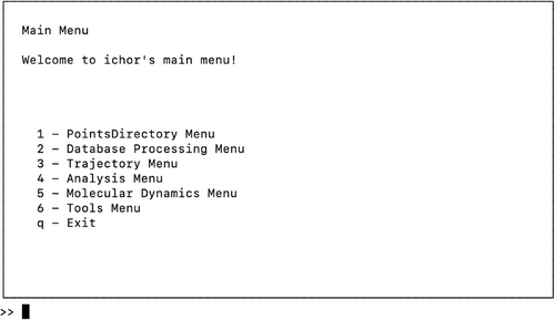
It is impossible for the CLI to contain all the functionalities implemented in ichor.core and ichor.hpc packages because this arrangement would overcomplicate the menu system and reduce its usefulness. Additionally, some calculations are impractical to carry out through the menus, in which case one has to resort back to using the full ichor library. For advanced options and more granularity, it is best to import relevant code from the ichor library into Python scripts and modify the calculation settings as needed.

5 MACHINE LEARNING FORCE FIELD TOOLS

As mentioned previously, ichor was designed to aid with ML force field development. Ichor has streamlined the process of molecular geometry generation, submission of first principles calculations, and data post-processing, allowing one to purely focus on the ML algorithms instead. Ichor has been an invaluable tool for the development of the in-house FFLUX⁵⁸ force field, which makes use of Gaussian process regression (GPR) for prediction of atomic energies and forces. Ichor does not have ML model-making functionality because the code focuses on data generation and analysis. Yet, there are many tools available in ichor for pre-processing of data for ML usage, as well performance benchmarking tools for ML models.

5.1 Featurization

Raw data from calculations can be easily obtained through ichor, as seen previously, but it is almost always the case that the data needs to be processed further before they can be utilized for ML purposes. This is because descriptors (also known as features), which are used as inputs to ML, are typically a function of the atomic coordinates of a set of atoms. Cartesian atomic coordinates are not used directly as ML inputs because of advantageous properties of the featurization, such as rotational and translational invariance, which simplify the modeling problem at hand. A potential energy surface can then be fitted via the selected descriptors through ML methods.

Ichor currently implements the atomic local frame (ALF) featurization,⁵⁹ which is what is used by FFLUX. This featurization maps atomic coordinates onto an internal coordinate frame. The resulting ALF features are a collection of distances and angles, which are invariant to global translations and rotations of a molecule in three-dimensional space. It is important to note that because the FFLUX models are currently atom-based, an ALF is defined for each individual atom in the (chemical) system, which leads to a different set of descriptors for each atom, depending on the chosen ALF.

An ALF can be defined by any three atoms in the system (containing more than two atoms). Currently two algorithms are implemented in ichor, which allow for the ALF determination. The first algorithm is based on the familiar Cahn-Ingold-Prelog priority rules. First atomic connectivity is determined (based on distance criteria) followed by the priorities of the atoms (i.e. which atom is the x-axis atom and which is the xy-plane atom). The second algorithm provides a simpler approach and is the default ALF determination method in ichor. This algorithm is simply based on the atom sequence in a file containing atomic coordinates. Figure 4 shows an example of how the algorithm works as described in detail in its caption.

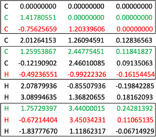
An advantage of the ALF sequence approach when compared to the previous Cahn-Ingold-Prelog approach is that the connectivity of the atoms is irrelevant and no distance criterion needs to be established. However, as expected, the sequence of the atoms is very important because changes in the sequence result in changes of the ALF definitions. There are many algorithms by which an ALF for an atom can be established, but what is more important is that the ALF definition for an atom remains the same across all molecular geometries. Using multiple ALF definitions for the same atom across molecular geometries yields different sets of ALF descriptors that will cause issues with the ML model predictions. The calculated connectivity may change in a scenario where geometries are very distorted, which will result in several different ALF definitions across geometries if the Cahn-Ingold-Prelog algorithm is used. However, in the sequence case, two very distorted geometries will still have the same ALFs as long as the sequence in the xyz file is the same.

After an ALF is determined for a given central atom, the ALF features for that central atom can be calculated. There are

3 N_{atoms} - 6

ALF features that give an exact representation of the molecular geometry through a local frame with the central atom positioned at the origin. Here we provide only a brief overview of the ALF feature calculations because more details can be found elsewhere.^{47, 59} The first three features are: (i) the distance from the central atom (with Cartesian coordinates

a

) to the x-axis atom (with coordinates

a_{x}

), (ii) the distance from the central atom to the xy-plane atom (with coordinates

a_{xy}

), and (iii) the angle between the x-axis atom, the central atom and the xy-plane atom. The rest of the atoms or so-called non-ALF atoms (that is, excluding the three atoms defining the ALF), are described by spherical polar coordinates with respect to the defined ALF coordinate system. Therefore, each non-ALF atom is described by three features: a distance from the origin

a_{n}

, polar angle

θ^{A_{n}}

, and azimuthal angle

ϕ^{A_{n}}

. The set of features can be calculated according to Equations (2-7),

a_{x} = ||a_{x} - a||,

(2)

a_{xy} = ||a_{xy} - a||,

(3)

χ^{A} = co s^{- 1} (\frac{a_{x} . a_{xy}}{a_{x} a_{xy}}),

(4)

a_{n} = ||a_{n} - a||,

(5)

θ^{A_{n}} = co s^{- 1} (\frac{ζ_{3}^{A_{n}}}{a_{n}}),

(6)

ϕ^{A_{n}} = ta n^{- 1} (\frac{ζ_{2}^{A_{n}}}{ζ_{1}^{A_{n}}}),

(7)

where

n = (4, \dots, N_{atoms})

and

N_{atoms}

is the number of atoms in the system. There are a total of

3 N_{atoms} - 6

ALF features for a non-linear system. The

ζ_{i}^{A_{n}}

component is the

i

-th local Cartesian component of atom

A_{n}

(calculated from the Cartesian ALF coordinate frame).

Although the current ichor code makes heavy use of the ALF featurization (because the code was initially developed to be used solely with FFLUX), the code is written in a modular way and allows for implementation of other featurization schemes. Custom functions that calculate atomic or molecular descriptors can be easily interfaced with ichor. A trivial example is shown just below where a Coulomb matrix⁶⁰ is constructed from a given geometry:

>>> from ichor.core.atoms import Atoms, Atom

>>> from ichor.core.common.constants import type2nuclear_charge

>>> import numpy as np

>>> def coulomb_matrix_representation(atoms: Atoms):

>>> …. natoms = len(atoms)

>>> …. res = np.empty((natoms, natoms))

>>> …. for i, atm1 in enumerate(atoms):

>>> …. …. for j, atom2 in enumerate(atoms):

>>> …. …. …. if i == j:

>>> …. …. …. …. res[i, j] = 0.5 * type2nuclear_charge[atm1.type]**2.4

>>> …. …. …. else:

>>> …. …. …. …. dist = np.linalg.norm(atm2.coordinates – atm1.coordinates)

>>> …. …. …. …. atm1_charge = type2nuclear_charge[atm1.type]

>>> …. …. …. …. atm2_charge = type2nuclear_charge[atm2.type]

>>> …. …. …. …. res[i, j] = (atm1_charge * atm2_charge) / dist

>>> …. return res

>>>

>>> atoms = Atoms([Atom("O", 0.0, 0.0, 0.0), Atom("H", 0.82, 0.0, 0.0), Atom("H", -0.54, 0.83, 0.0)])

>>> coulomb_matrix = atoms.features(coulomb_matrix_representation, is_atomic=False)

>>> coulomb_matrix

[[73.51669472 9.75609756 8.07915961]
[ 9.75609756 0.5 0.62764116]
[ 8.07915961 0.62764116 0.5 ]]

5.2 ALF forces

Most ML models designed for molecular simulations incorporate atomic forces into the model architecture. Currently, FFLUX does not utilize derivative information into the GPR models of atomic energies or atomic multipole moments. Although energy based GPR models can be differentiated to obtain forces, it is possible to directly incorporate derivative information in the GPR models. There exists literature that discusses incorporating derivative information in GPR models, specifically for the purpose of simulations.^61-64

Typically, electronic structure calculation code, which is used to make datasets for ML force field development, readily calculates the derivatives of the potential energy surface. However, analytical Cartesian forces obtained from computational chemistry software cannot be used directly in the FFLUX GPR models because they use ALF features as inputs. A coordinate transformation is therefore needed from Cartesian coordinates to ALF coordinates, which can be performed by a method proposed by Pulay and Fogarasi.⁶⁵ The coordinate transformation is carried out by first forming the

B

matrix,⁶⁶ containing elements

B_{ij}

shown in Equation (8),

B_{ij} = \frac{\partial f_{i}}{\partial c_{j}},

(8)

which are the derivatives of the ALF features

f_{i}

with respect to the Cartesian coordinates

c_{j}

. These derivatives have already been covered in detail in previous work.⁵⁹ The

B

matrix is of size

(3 N_{atoms} - 6) \times 3 N_{atoms}

. Note that the ALF features contain the minimum number of coordinates required to fully describe a system. Therefore, there are no redundant ALF features, and hence all rows of the

B

matrix are linearly independent.

To transform the Cartesian forces to feature forces, the

G

matrix is formed according to Equation (9),

G = B B^{T},

(9)

and the energy gradient

g_{f}

in ALF feature coordinates is calculated as

g_{f} = G^{- 1} B g_{c},

(10)

where the vector

g_{c}

contains all

3 N_{atoms}

forces for all atoms. Care must be taken to ensure that the vector

g_{c}

contains the correct sequence of the Cartesian forces because the

B

matrix rows will be in the order of the ALF features, which might order the ALF coordinates of the atoms in a different way. As the rows of

B

are linearly independent

B B^{T}

is guaranteed to have an inverse. Additionally, the

G

matrix is a symmetric square matrix and positive semidefinite, so Cholesky decomposition can be used to efficiently solve for

g_{f}

by forward and backward substitution. The ALF coordinates gradient

g_{f}

can be readily transformed back to Cartesian coordinates by Equation (11),

g_{c} = B^{T} g_{f} .

(11)

The ML models will require the gradient vector instead of the force vector. Since computational chemistry programs output the Cartesian forces instead of the gradient, one needs the additional step of taking the negative of the analytical force vector in Cartesian forces

f_{c}

to obtain the gradient of the potential energy surface in Cartesian coordinates

g_{c}

, as shown in Equation (12),

g_{c} = - f_{c} .

(12)

The equations presented above are already implemented in ichor and one can readily obtain ML datasets that include derivative information. GPR models with derivative information that utilize ALF featurization are currently being tested. More details on the implementation of the actual GPR models will be presented in future work.

5.3 Dataset visualization

Most molecular geometries collected in ML datasets have been created by ab initio molecular dynamics (MD) or by simulations with molecular-mechanics-based FFs. It is very useful to understand the configuration space of geometries contained in the dataset because ML models that use an improperly constructed dataset are unlikely to perform well in MD simulations, even if the models predict test data properties well. If the test data are obtained from an improperly sampled dataset, then the test data may not contain all the necessary information that will make the model suitable for simulations. Therefore, predicting well on the test data may not translate to well performing simulations.

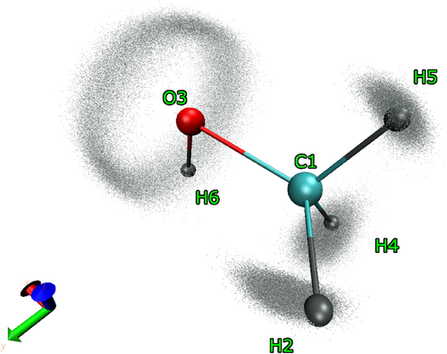
ALF features can be readily converted back into Cartesian coordinates and allow for reconstruction of the original molecular geometry, without any information loss. Converting ALF features for multiple geometries back into Cartesian coordinates effectively centers different molecular configurations on the local coordinate frame defined for the atom. To achieve this, a central atom, x-axis atom, and xy-plane atoms are selected, and the ALF features associated with the central atom are calculated. The ALF features are converted back to Cartesian coordinates and the centered geometries can be visualized. For example, Figure 5 shows a centered methanol trajectory using the ALF centering scheme to create so-called “mist plots.” The image is created by plotting all steps of a trajectory as the “points” representation and an example geometry with the CPK representation in the VMD⁶⁷ program. As can be seen, all atom movements are mapped onto the ALF coordinate system. The central ALF atom always stays in the same position. The x-axis atom moves only along a line, while the xy-plane atom only moves in a plane. All movements of other atoms are mapped with respect to the pre-defined local coordinate system.

5.4 GPR predictions

GPR is one of the cornerstones of FFLUX. Ichor itself does not have the capability to make GPR models but it does have the ability to make predictions (of both energy and forces) utilizing already created GPR models. This functionality is required to test model performance prior to deploying them in FFLUX MD simulations. The GPR models themselves are made by other pieces of software such as the in-house Fortran90 program FEREBUS^68-70 and more recently by the GPyTorch⁷¹ package. The general equation for making GPR predictions is shown in Equation 13,

\bar{f} (x^{*}) = k (x^{*}, X) α + μ (x^{*}) .

(13)

where

k (x^{*}, X)

is the covariance vector between a test point

x^{*}

(for which a prediction is being made) and the training dataset

X

, while

α

is the weights vector, and

μ

is a prior mean. Note that the prior mean can be any function, including a constant value function (which is typically what is used in the GPR models). The weights vector

α

is completely pre-determined by the training set, and is calculated by Equation (14),

{[k (X, X) + σ^{2} I]}^{- 1} (y - μ) = α,

(14)

where

k (X, X)

indicates the covariance matrix between each two training set points, with added noise

σ^{2}

on the diagonal, while

y

is the vector containing the training labels, and

μ

is the prior mean vector. The prior mean vector contains the prior mean at all training points

x

, and in this case contains the same (constant) element

μ

. Since

α

only depends on the training set, it can be cached and used when predictions are needed on a new test point.

Ichor implements the Model Python class, which is used to parse GPR model files, containing all necessary information to make predictions on a test point. The GPR model files are based on the TOML file format, and a general structure of model files can be found in the Section 8 of the SI. FFLUX itself also uses the model files to make predictions during an MD simulation. To make predictions, ichor implements the RBF and periodic kernels because these are the current kernel functions utilized in FFLUX. The RBF kernel is written according to Equation (15),

k_{rbf} (x, x^{'}) = τ_{rbf}^{2} \exp (- \sum_{d} \frac{{(x_{d} - x_{d}^{'})}^{2}}{2 l_{d}^{2}}),

(15)

and the periodic kernel is written according to Equation (16),

k_{per} (x, x^{'}) = τ_{per}^{2} \exp (- 2 \sum_{e} \frac{\sin^{2} (π (x_{e} - x_{e}^{'}) / p_{e})}{l_{e}^{2}}),

(16)

where

l_{d}

and

l_{e}

are lengthscale hyperparameters, and

p_{e}

is a period length hyperparameter. The period length is known and set to

2 π

for all

e

dimensions (which are the dimensions of

ϕ

ALF features), as the covariance repeats every

2 π

in these dimensions. The outputscale hyperparameter

τ

is a scaling factor for GPR model variance and has no effect on model predictions. Therefore, the value of

τ

is set to 1 for both kernels when making the model files, as well as when making predictions with the model files.

Ichor can directly predict properties, such as energy and forces from the GPR models of any system. The prediction code can be readily modified to accept new kernels, and a powerful interpreter has been written to detect which kernels are used in the model files. The interpreter automatically determines operations applied to a set of kernels, such as addition or multiplication of kernels, making it straightforward to change the kernel structure or combine different kernels. At the moment, the model files are tied with the ALF featurization scheme but they can be modified to accommodate any featurization if needed.

5.5 Model benchmarking

Standardized benchmarking tools are critical for advancements and comparison of machine learning force fields. There are two separate ways that ML models made for molecular simulations can be benchmarked. The first way is to predict atomic and molecular properties, such as energy and forces on a given test set that is outside of the scope of the training set used to make the ML model. While this is a standard way of benchmarking model prediction accuracy it is not optimal: even good test set prediction accuracy may give an incorrect indication on how the model will perform in simulation. Therefore, the second approach, which is to run an MD simulation using the given ML models, presents a more suitable test that clearly signals if the ML models are good enough. Ichor does not provide the tools to run MD simulations but it does provide metrics for checking simulation stability and robustness after simulations are ran. The following five subsections give an overview of the tools that ichor implements for model benchmarking. Although some of the functionalities are specifically tied in with FFLUX's development, others are much more general and can be used for development of any ML force field.

5.5.1 S-curves

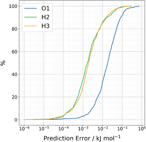
S-curves have been extensively used in our own work^72-75 as they allow one to gauge model prediction quality on test sets. Figure 6 shows an example of an S-curve where the absolute prediction error is plotted against a percentile, with the maximum absolute prediction error for a test point reached at the hundredth percentile. S-curves are a very general tool and are agnostic to the property that is being predicted, so they can be used to test prediction accuracy for total system energies and atomic multipole moments as well. Additionally, S-curves are agnostic to where the test geometries were obtained from: the test geometries can either be obtained from a set of geometries not used for training the GPR models or extracted from MD simulations with the GPR models. S-curves are typically accompanied by metrics such as Root Mean Square Error (RMSE) and Mean Absolute Error (MAE), which provide general guidance on the predictive power of the ML model. The further the S-curves are shifted to the left the better as this indicates a lower absolute prediction error for the test data. Note that coordination number and atomic volumes do increase the numerical noise in atomic property calculations, which results in S-curves of heavier atoms being shifted to the right when compared to hydrogen atom S-curves.

5.5.2 True versus predicted plots

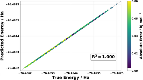
The GPR models predict energies and forces throughout the simulation, which can be compared to GAUSSIAN reference calculations. First, one can compare the predicted energy versus the reference energy, both for the total system, as calculated by GAUSSIAN. Figure 7 shows the true versus predicted energies, which can be obtained directly from ichor. It is also possible to use this type of plot without MD simulations, as it is also perfectly suitable to use it for test sets that do not come from simulations with the ML models.

5.5.3 Mean absolute error of forces plots

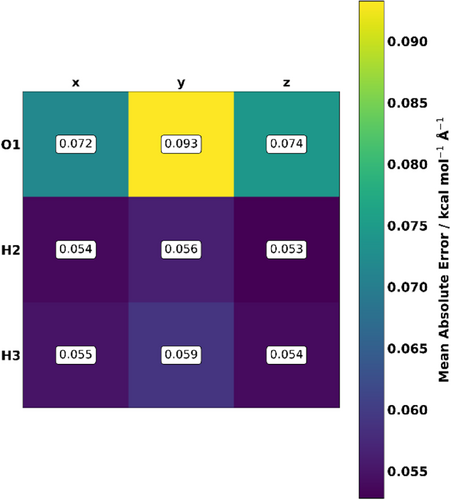
Additionally, the force prediction accuracy of models can be gauged by plotting a matrix, showing the MAE prediction errors in the x, y and z directions for the whole MD simulation. Figure 8 shows an example plot for a water monomer model. Plots like these allow one to notice patterns in force prediction accuracy of certain atoms, as well as directly quantify the quality of force predictions during a simulation. Similarly to the true-versus-predicted plot these force plots can also be made for test set data without simulations. However, it is better to utilize these in simulations, because predictions on a test set sometimes do not translate to good model-performance in MD simulations.

5.5.4 Distribution of interatomic distances plots

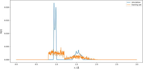
It is important to get a sense of how much atoms move in a simulation. Hence, we implemented the distribution of interatomic distances, as proposed by Fu et al.⁴⁴ Essentially, the proposed algorithm counts the number of interatomic distances that fall within a certain distance range, into bins based on interatomic distance $r$ and calculates the function $h (r)$ . Figure 9 shows an example plot comparing $h (r)$ calculated for a water monomer FFLUX simulation and the training set from which are constructed the GPR models used in the simulation. There are two main observations that can be taken away from a plot like this. First, the plot shows how much interatomic distances between atoms change throughout a simulation, and the peaks can be assigned to specific interactions for simple molecules. For example, the first set of peaks occurring at around 1 Å is a result of the oxygen-hydrogen bond distance, while the second set around 1.5 Å is a result of the hydrogen–hydrogen distance. Second, it can be clearly seen from the plot that the training set covers a wider range of interatomic distances compared to that of the 298 K FFLUX simulation, meaning that the training set is adequate for the current simulation. Of course, changing the temperature of simulation will result in a different distribution of distances. Similar monitoring for the angle changes will also be implemented in future ichor releases to be able to analyze angular movements as well.

5.5.5 Energy versus timestep plots

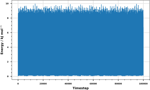
The fifth and last benchmarking tool that ichor currently provides enables plotting the energy of the system as an MD simulation progresses, an example of which can be seen in Figure 10. Such plots are useful for checking if a simulation has equilibrated or, in the case of a geometry optimization, to check if the energy is converging towards a minimum. Additionally, these plots allow for comparison of the deviation between the energy for the optimized geometry and the energy of the geometries generated throughout the MD simulation. These plots can be used to compare predicted energies across different simulation runs (with different velocity seeds, for example).

5.6 Multipole moment calculations

Ichor is able to convert between spherical and Cartesian multipole moments, as described by Stone,⁷⁶ as well as to rotate multipole moments up to and including the hexadecapole moment. This functionality is required because FFLUX incorporates electrostatics using atomic multipole moments (up to and including the hexadecapole moment). FFLUX uses the spherical harmonic formalism for multipole moments because it eliminates the redundancies that are present in the Cartesian representation. In order to make the ML models compatible with FFLUX, the atomic multipole moments calculated by AIMAll need to be rotated into the local coordinate system defined by an ALF. While it is possible to directly learn the multipole moments in the global coordinate system that AIMAll uses, doing so is sub-optimal because the rotations would then need to be done in FFLUX for each timestep, which requires additional unnecessary computations. Rotating the multipole moments prior to model training makes the FFLUX prediction code more efficient.

Additionally, while it is possible to compare the atomic multipole moments predicted by the GPR models to AIMAll reference data, no testing has so far been carried out on the recovery of the molecular multipole moments in FFLUX MD simulations. The correct recovery of the molecular multipole moment from atomic ones is an important next step in ensuring predicted multipole moments are in line with reference data. Ichor implements all necessary equations thereby allowing one to recover the molecular dipole and quadrupole moments from atomic dipole and quadrupole moments, respectively. The equations for the conversion from atomic to molecular multipole moments have already been published previously.⁷⁷ Furthermore, ichor implements functions that calculate multipole moments given an origin change. Details of these calculations, as well as extensions of the equations to octupole and hexadecapole moments, will be presented in a follow-up paper discussing multipole moment calculations and conversions. In addition, the reconstruction accuracy of molecular multipole moments from atomic ones will be benchmarked for the first time for systems of various sizes and chemical structures.

6 CONCLUSIONS

We introduced ichor, a Python package that drastically improves data management for computational chemistry tasks, and specifically intended to aid machine learning force field development. The ichor code base implements a very robust and readily extensible data management system, which can be interfaced with popular third-party Python libraries for file parsing. The ichor data structures include several layers, ranging from single-file handling classes to classes that simultaneously handle thousands of files. The high-level data structures allow one to easily obtain information from many separate calculations at once. Raw data can be conveniently stored into databases, making postprocessing and sharing of data much easier. Ichor also implements interfaces to workflow management software on HPC clusters, allowing submission of thousands of calculations with a single line of Python code. The HPC interfaces are easily modifiable to accept new computational chemistry workflows. With the functionalities above, ichor can be used as an all-in-one solution for dataset generation for machine learning force field development.

In addition to general purpose data handling tools, ichor has a great amount of functionality relating to the benchmarking of machine learning models. Although some of the current functionality is inherently tied in with FFLUX, most of the analysis tools are general enough to find uses in other machine learning force field frameworks. The ultimate tests for machine learning models are simulations, and both accuracy as well as simulation stability of these models need to be rigorously tested. As the ichor code matures, additional benchmarking tools will be added, which will give more ways to assess machine learning model and simulation performance.

This release of ichor contains the essential functionalities that drastically increase productivity for computational chemistry tasks and machine learning force field development. As the code base matures, more functionalities relating to data management and processing, as well machine learning model and MD simulation analysis will be added. We hope that the current code base can be used in many different computational chemistry workflows and encourage anyone interested in the code base to contribute. The ichor code is completely free to use and open source. We hope that ichor finds uses in the wider research community and enables research to be done in a more efficient and reproducible manner.

ACKNOWLEDGMENTS

Y.T.M. acknowledges the (UKRI) BBSRC DTP for the award of a PhD studentship while P.L.A.P is grateful to the European Research Council (ERC) for the award of an Advanced Grant underwritten by the UKRI-funded Frontier Research grant EP/X024393/1. Y.T.M. thanks Fabio Falcioni for the initial implementation of the interatomic distances analysis tool.

Open Research

DATA AVAILABILITY STATEMENT

Ichor is fully free and open-source software available under the MIT license. The ichor code, along with examples and documentation, can be found at https://github.com/popelier-group/ichor. Contributions to the project are very welcome, please refer to the contribution guidelines for more information.

Supporting Information

REFERENCES

1M. Kowalewski, P. Seeber, Int. J. Quantum Chem. 2022, 122, e26872.
10.1002/qua.26872
CAS Web of Science® Google Scholar
2V. Gavini, S. Baroni, V. Blum, D. R. Bowler, A. Buccheri, J. R. Chelikowsky, S. Das, W. Dawson, P. Delugas, M. Dogan, C. Draxl, G. Galli, L. Genovese, P. Giannozzi, M. Giantomassi, X. Gonze, M. Govoni, F. Gygi, A. Gulans, J. M. Herbert, S. Kokott, T. D. Kühne, K.-H. Liou, T. Miyazaki, P. Motamarri, A. Nakata, J. E. Pask, C. Plessl, L. E. Ratcliff, R. M. Richard, M. Rossi, R. Schade, M. Scheffler, O. Schütt, P. Suryanarayana, M. Torrent, L. Truflandier, T. L. Windus, Q. Xu, V. W. Z. Yu, D. Perez, Modell. Simul. Mater. Sci. Eng. 2023, 31, 63301.
10.1088/1361-651X/acdf06
Google Scholar
3Y. Shao, L. F. Molnar, Y. Jung, J. Kussmann, C. Ochsenfeld, S. T. Brown, A. T. B. Gilbert, L. V. Slipchenko, S. V. Levchenko, D. P. O'Neill, R. A. DiStasio, R. C. Lochan, T. Wang, G. J. O. Beran, N. A. Besley, J. M. Herbert, C. Yeh Lin, T. Van Voorhis, S. Hung Chien, A. Sodt, R. P. Steele, V. A. Rassolov, P. E. Maslen, P. P. Korambath, R. D. Adamson, B. Austin, J. Baker, E. F. C. Byrd, H. Dachsel, R. J. Doerksen, A. Dreuw, B. D. Dunietz, A. D. Dutoi, T. R. Furlani, S. R. Gwaltney, A. Heyden, S. Hirata, C. P. Hsu, G. Kedziora, R. Z. Khalliulin, P. Klunzinger, A. M. Lee, M. S. Lee, W. Liang, I. Lotan, N. Nair, B. Peters, E. I. Proynov, P. A. Pieniazek, Y. Min Rhee, J. Ritchie, E. Rosta, C. David Sherrill, A. C. Simmonett, J. E. Subotnik, H. Lee Woodcock, W. Zhang, A. T. Bell, A. K. Chakraborty, D. M. Chipman, F. J. Keil, A. Warshel, W. J. Hehre, H. F. Schaefer, J. Kong, A. I. Krylov, P. M. W. Gill, M. Head-Gordon, Phys. Chem. Chem. Phys. PCCP 2006, 8, 3172.
10.1039/B517914A
CAS PubMed Web of Science® Google Scholar
4A. V. Sadybekov, V. Katritch, Nature 2023, 616, 673.
10.1038/s41586-023-05905-z
CAS PubMed Web of Science® Google Scholar
5N. Schaduangrat, S. Lampa, S. Simeon, M. P. Gleeson, O. Spjuth, C. Nantasenamat, J. Cheminform. 2020, 12, 1.
10.1186/s13321-020-0408-x
PubMed Google Scholar
6W. L. Jorgensen, Science 2004, 303, 1813.
10.1126/science.1096361
CAS PubMed Web of Science® Google Scholar
7P. M. Fischer, Biotechnol. J. 2008, 3, 452.
10.1002/biot.200700259
CAS PubMed Google Scholar
8S.-S. Ou-Yang, J.-Y. Lu, X.-Q. Kong, Z.-J. Liang, C. Luo, H. Jiang, Acta Pharmacol. Sin. 2012, 33, 1131.
10.1038/aps.2012.109
CAS PubMed Web of Science® Google Scholar
9M. Pandey, M. Fernandez, F. Gentile, O. Isayev, A. Tropsha, A. C. Stern, A. Cherkasov, Nat. Mach. Intell. 2022, 4, 211.
10.1038/s42256-022-00463-x
Google Scholar
10L. Frye, S. Bhat, K. Akinsanya, R. Abel, Drug Discov. Today Technol. 2021, 39, 111.
10.1016/j.ddtec.2021.08.001
CAS PubMed Google Scholar
11M. Steinhauser, S. Hiermaier, Int. J. Mol. Sci. 2009, 10, 5135.
10.3390/ijms10125135
CAS PubMed Web of Science® Google Scholar
12J. Neugebauer, T. Hickel, WIREs Comput. Mol. Sci. 2013, 3, 438.
10.1002/wcms.1125
CAS PubMed Web of Science® Google Scholar
13A. J. Freeman, E. Wimmer, Annu. Rev. Mater. Sci. 1995, 25, 7.
10.1146/annurev.ms.25.080195.000255
CAS Web of Science® Google Scholar
14J. Hafner, C. Wolverton, G. Ceder, MRS Bull. 2006, 31, 659.
10.1557/mrs2006.174
Web of Science® Google Scholar
15R. Gómez-Bombarelli, A. Aspuru-Guzik. Springer International Publishing: 2020, p 1939.
Google Scholar
16P. Selvam, H. Tsuboi, M. Koyama, A. Endou, H. Takaba, M. Kubo, C.A. Del Carpio, A. Miyamoto, 2006, 22, 377.
Google Scholar
17B. W. J. Chen, L. Xu, M. Mavrikakis, Chem. Rev. 2021, 121, 1007.
10.1021/acs.chemrev.0c01060
CAS PubMed Web of Science® Google Scholar
18X. Zhang, L. W. Chung, Y.-D. Wu, Acc. Chem. Res. 2016, 49, 1302.
10.1021/acs.accounts.6b00093
CAS PubMed Web of Science® Google Scholar
19W. Thiel, Angew. Chem. Int. Ed. 2014, 53, 8605.
10.1002/anie.201402118
CAS PubMed Web of Science® Google Scholar
20M. G. Quesne, F. Silveri, N. H. de Leeuw, C. R. A. Catlow, Front. Chem. 2019, 7, 1.
10.3389/fchem.2019.00182
PubMed Google Scholar
21K. D. Vogiatzis, M. V. Polynski, J. K. Kirkland, J. Townsend, A. Hashemi, C. Liu, E. A. Pidko, Chem. Rev. 2019, 119, 2453.
10.1021/acs.chemrev.8b00361
CAS PubMed Web of Science® Google Scholar
22M. J. Ramos, P. A. Fernandes, Acc. Chem. Res. 2008, 41, 689.
10.1021/ar7001045
CAS PubMed Web of Science® Google Scholar
23G. A. McCarver, T. Rajeshkumar, K. D. Vogiatzis, Coord. Chem. Rev. 2021, 436, 213777.
10.1016/j.ccr.2021.213777
CAS Web of Science® Google Scholar
24J. K. Nørskov, T. Bligaard, J. Rossmeisl, C. H. Christensen, Nat. Chem. 2009, 1, 37.
10.1038/nchem.121
CAS PubMed Web of Science® Google Scholar
25N. Fey, Dalton Trans. 2010, 39, 296.
10.1039/B913356A
CAS Web of Science® Google Scholar
26S. Martí, M. Roca, J. Andrés, V. Moliner, E. Silla, I. Tuñón, J. Bertrán, Chem. Soc. Rev. 2004, 33, 98.
10.1039/B301875J
CAS PubMed Web of Science® Google Scholar
27P. G. Tratnyek, E. J. Bylaska, E. J. Weber, Environ. Sci. Process. Impacts 2017, 19, 188.
10.1039/C7EM00053G
CAS PubMed Web of Science® Google Scholar
28L. Sviatenko, O. Isayev, L. Gorb, F. Hill, J. Leszczynski, J. Comput. Chem. 2011, 32, 2195.
10.1002/jcc.21803
CAS PubMed Web of Science® Google Scholar
29S. Lehtola, J. Chem. Phys. 2023, 159, 1.
Google Scholar
30S. Lehtola, A. J. Karttunen, Wiley Interdiscip. Rev. Comput. Mol. Sci. 2022, 12, 1.
10.1002/wcms.1610
Google Scholar
31R. Di Felice, M. L. Mayes, R. M. Richard, D. B. Williams-Young, G. K.-L. Chan, W. A. de Jong, N. Govind, M. Head-Gordon, M. R. Hermes, K. Kowalski, X. Li, H. Lischka, K. T. Mueller, E. Mutlu, A. M. N. Niklasson, M. R. Pederson, B. Peng, R. Shepard, E. F. Valeev, M. van Schilfgaarde, B. Vlaisavljevich, T. L. Windus, S. S. Xantheas, X. Zhang, P. M. Zimmerman, J. Chem. Theory Comput. 2023, 19, 7056.
10.1021/acs.jctc.3c00419
CAS PubMed Google Scholar
32N. M. O'Boyle, A. L. Tenderholt, K. M. Langner, J. Comput. Chem. 2008, 29, 839.
10.1002/jcc.20823
CAS PubMed Web of Science® Google Scholar
33T. Verstraelen, W. Adams, L. Pujal, A. Tehrani, B. D. Kelly, L. Macaya, F. Meng, M. Richer, R. Hernández-Esparza, X. D. Yang, M. Chan, T. D. Kim, M. Cools-Ceuppens, V. Chuiko, E. Vöhringer-Martinez, P. W. Ayers, F. Heidar-Zadeh, J. Comput. Chem. 2021, 42, 458.
10.1002/jcc.26468
CAS PubMed Web of Science® Google Scholar
34S. P. Ong, W. D. Richards, A. Jain, G. Hautier, M. Kocher, S. Cholia, D. Gunter, V. L. Chevrier, K. A. Persson, G. Ceder, Comput. Mater. Sci. 2013, 68, 314.
10.1016/j.commatsci.2012.10.028
CAS Web of Science® Google Scholar
35N. M. O'Boyle, M. Banck, C. A. James, C. Morley, T. Vandermeersch, G. R. Hutchison, J. Cheminform. 2011, 3, 33.
10.1186/1758-2946-3-33
CAS PubMed Web of Science® Google Scholar
36M. D. Wilkinson, M. Dumontier, I. J. Aalbersberg, G. Appleton, M. Axton, A. Baak, N. Blomberg, J.-W. Boiten, L. B. da Silva Santos, P. E. Bourne, J. Bouwman, A. J. Brookes, T. Clark, M. Crosas, I. Dillo, O. Dumon, S. Edmunds, C. T. Evelo, R. Finkers, A. Gonzalez-Beltran, A. J. G. Gray, P. Groth, C. Goble, J. S. Grethe, J. Heringa, P. A. C. Hoen, T. K. Hooft, R. Kok, J. Kok, S. J. Lusher, M. E. Martone, A. Mons, A. L. Packer, B. Persson, P. Rocca-Serra, M. Roos, R. van Schaik, S.-A. Sansone, E. Schultes, T. Sengstag, T. Slater, G. Strawn, M. A. Swertz, M. Thompson, J. van der Lei, E. van Mulligen, J. Velterop, A. Waagmeester, P. Wittenburg, K. Wolstencroft, J. Zhao, B. Mons, Sci. Data 2016, 3, 160018.
10.1038/sdata.2016.18
PubMed Web of Science® Google Scholar
37A. Hjorth Larsen, J. Jørgen Mortensen, J. Blomqvist, I. E. Castelli, R. Christensen, M. Duak, J. Friis, M. N. Groves, B. Hammer, C. Hargus, E. D. Hermes, P. C. Jennings, P. B. Jensen, J. Kermode, J. R. Kitchin, E. L. Kolsbjerg, J. Kubal, K. Kaasbjerg, S. Lysgaard, J. B. Maronsson, T. Maxson, T. Olsen, L. Pastewka, A. Peterson, C. Rostgaard, J. Schiøtz, O. Schütt, M. Strange, K. S. Thygesen, T. Vegge, L. Vilhelmsen, M. Walter, Z. Zeng, K. W. Jacobsen, J. Phys. Conden. Matter 2017, 29, 273002.
10.1088/1361-648X/aa680e
PubMed Web of Science® Google Scholar
38K. Mathew, J. H. Montoya, A. Faghaninia, S. Dwarakanath, M. Aykol, H. Tang, I. H. Chu, T. Smidt, B. Bocklund, M. Horton, J. Dagdelen, B. Wood, Z.-K. Liu, J. Neaton, S. P. Ong, K. Persson, A. Jain, Comput. Mater. Sci. 2017, 139, 140.
10.1016/j.commatsci.2017.07.030
Web of Science® Google Scholar
39A. Jain, S. P. Ong, W. Chen, B. Medasani, X. Qu, M. Kocher, M. Brafman, G. Petretto, G.-M. Rignanese, G. Hautier, D. Gunter, K. A. Persson, Concurr. Comput. 2015, 27, 27.
10.1002/cpe.3505
Google Scholar
40M. Handzlik, SCM: Amsterdam 2019.
Google Scholar
41L. Himanen, M. O. J. Jäger, E. V. Morooka, F. Federici Canova, Y. S. Ranawat, D. Z. Gao, P. Rinke, A. S. Foster, Comput. Phys. Commun. 2020, 247, 106949.
10.1016/j.cpc.2019.106949
CAS Web of Science® Google Scholar
42J. Laakso, L. Himanen, H. Homm, E. V. Morooka, M. O. J. Jäger, M. Todorović, P. Rinke, J. Chem. Phys. 2023, 158, 234802.
10.1063/5.0151031
CAS PubMed Google Scholar
43G. Landrum 2010.
Google Scholar
44X. Fu, Z. Wu, W. Wang, T. Xie, S. Keten, R. Gomez-Bombarelli, T. Jaakkola, Trans. Mach. Learn. Res. 2022, 1, 1.
Google Scholar
45P. Maxwell, N. Di Pasquale, S. Cardamone, P. L. A. Popelier, Theor. Chem. Acc. 2016, 135, 135.
10.1007/s00214-016-1951-4
Google Scholar
46T. L. Fletcher, S. J. Davie, P. L. A. Popelier, J. Chem. Theory Comput. 2014, 10, 3708.
10.1021/ct500416k
CAS PubMed Web of Science® Google Scholar
47M. J. Burn, P. L. A. Popelier, Mater. Adv. 2022, 3, 8729.
10.1039/D2MA00673A
Google Scholar
48D. A. Case, T. E. Cheatham, C. L. Simmerling, J. Wang, R. E. Duke, K. M. M. Luo, D. A. Pearlman, M. Crowley, R. C. Walker, W. Zhang, B. Wang, A. R. Hayik, G. Seabra, K. F. Wong, F. Paesani, X. Wu, S. Brozell, V. Tsui, L. Y. Gohlke, C. Tan, J. Mongan, V. Hornak, G. Cui, P. Beroza, D. H. Mathews, W. S. R. Schafmeister, P. A. Kollman, AMBER 9, University of California, San Francisco 2006.
Google Scholar
49T. D. Kühne, M. Iannuzzi, M. Del Ben, V. V. Rybkin, P. Seewald, F. Stein, T. Laino, R. Z. Khaliullin, O. Schütt, F. Schiffmann, D. Golze, J. Wilhelm, S. Chulkov, M. H. Bani-Hashemian, V. Weber, U. Borštnik, M. Taillefumier, A. S. Jakobovits, A. Lazzaro, H. Pabst, T. Müller, R. Schade, M. Guidon, S. Andermatt, N. Holmberg, G. K. Schenter, A. Hehn, A. Bussy, F. Belleflamme, G. Tabacchi, A. Glöß, M. Lass, I. Bethune, C. J. Mundy, C. Plessl, M. Watkins, J. VandeVondele, M. Krack, J. Hutter, J. Chem. Phys. 2020, 152, 194103.
10.1063/5.0007045
CAS PubMed Web of Science® Google Scholar
50M. J. Frisch, H. B. S. G. W. Trucks, G. E. Scuseria, M. A. Robb, J. R. Cheeseman, G. Scalmani, V. Barone, G. A. Petersson, H. Nakatsuji, X. Li, M. Caricato, A. V. Marenich, J. Bloino, B. G. Janesko, R. Gomperts, B. Mennucci, H. P. Hratchian, J. V. Ortiz, A. F. Izmaylov, J. L. Sonnenberg, F. D. Williams, F. Lipparini, F. Egidi, J. Goings, B. Peng, A. Petrone, T. Henderson, D. Ranasinghe, V. G. Zakrzewski, J. Gao, N. Rega, G. Zheng, W. Liang, M. Hada, M. Ehara, K. Toyota, R. Fukuda, J. Hasegawa, M. Ishida, T. Nakajima, Y. Honda, O. Kitao, H. Nakai, T. Vreven, K. Throssell, J. A. Montgomery Jr., J. E. Peralta, F. Ogliaro, M. J. Bearpark, J. J. Heyd, E. N. Brothers, K. N. Kudin, V. N. Staroverov, T. A. Keith, R. Kobayashi, J. Normand, K. Raghavachari, A. P. Rendell, J. C. Burant, S. S. Iyengar, J. Tomasi, M. Cossi, J. M. Millam, M. Klene, C. Adamo, R. Cammi, J. W. Ochterski, R. L. Martin, K. Morokuma, O. Farkas, J. B. Foresman, D. J. Fox, GAUSSIAN16. 2016.
Google Scholar
51F. Neese, F. Wennmohs, U. Becker, C. Riplinger, J. Chem. Phys. 2020, 152, 224108.
10.1063/5.0004608
CAS PubMed Web of Science® Google Scholar
52P. L. A. Popelier, Int. J. Quant. Chem. 2015, 115, 1005.
10.1002/qua.24900
CAS Web of Science® Google Scholar
53I. T. Todorov, W. Smith, CCLRC Daresbury Laboratory, Daresbury Laboratory: Warrington, UK 2006.
Google Scholar
54T. A. Keith, AIMAll (Version 16.01.09), Overland Park, Kansas, USA. 2016.
Google Scholar
55K. Hinsen, Comput. Sci. Eng. 2009, 11, 86.
10.1109/MCSE.2009.129
Google Scholar
56M. A. Blanco, A. Martín Pendás, E. Francisco, J. Chem. Theory Comput. 2005, 1, 1096.
10.1021/ct0501093
CAS PubMed Web of Science® Google Scholar
57 aegirhall. 2018 https://github.com/aegirhall/console-menu
Google Scholar
58B. C. B. Symons, M. K. Bane, P. L. A. Popelier, J. Chem. Theor. Comp. 2021, 17, 7043.
10.1021/acs.jctc.1c00595
CAS PubMed Web of Science® Google Scholar
59M. J. L. Mills, P. L. A. Popelier, J. Chem. Theory Comput. 2014, 10, 3840.
10.1021/ct500565g
CAS PubMed Web of Science® Google Scholar
60M. Rupp, A. Tkatchenko, K.-R. Müller, O. A. von Lilienfeld, Phys. Rev. Lett. 2012, 108, 58301.
10.1103/PhysRevLett.108.058301
CAS PubMed Web of Science® Google Scholar
61A. Denzel, J. Kästner, J. Chem. Phys. 2018, 148, 94114.
10.1063/1.5017103
Web of Science® Google Scholar
62R. Lindh, I. Fdez, in Quantum Chemistry in the Age of Machine Learning (Ed: P. O. Dral), Elsevier, Oxford, UK. 2023, p. 391.
10.1016/B978-0-323-90049-2.00017-2
Google Scholar
63D. Born, J. Kästner, J. Chem. Theory Comput. 2021, 17, 5955.
10.1021/acs.jctc.1c00517
CAS PubMed Web of Science® Google Scholar
64S. Chmiela, A. Tkatchenko, H. E. Sauceda, I. Poltavsky, K. T. Schütt, K.-R. Müller, Sci. Adv., 2017, 3, e1603015.
10.1126/sciadv.1603015
PubMed Web of Science® Google Scholar
65P. Pulay, G. Fogarasi, J. Chem. Phys. 1992, 96, 2856.
10.1063/1.462844
CAS Web of Science® Google Scholar
66D. Wilson, J. Decius, C. Paul. McGraw-Hill, New York: 1955.
Google Scholar
67W. Humphrey, A. Dalke, K. Schulten, J. Mol. Graphics 1996, 14, 33.
10.1016/0263-7855(96)00018-5
CAS PubMed Web of Science® Google Scholar
68M. J. Burn, P. L. A. Popelier, Digital Discov. 2023, 2, 152.
10.1039/D2DD00082B
CAS Google Scholar
69N. Di Pasquale, M. Bane, S. J. Davie, P. L. A. Popelier, J. Comput. Chem. 2016, 37, 2606.
10.1002/jcc.24486
CAS PubMed Web of Science® Google Scholar
70B. K. Isamura, P. L. A. Popelier, Artif. Intell. Chem. 2023, 1, 100021.
10.1016/j.aichem.2023.100021
Google Scholar
71J. R. Gardner, G. Pleiss, D. Bindel, K. Q. Weinberger, A. G. Wilson, Conference on Neural Information Processing Systems Canada. 2018.
Google Scholar
72Y. T. Manchev, P. L. A. Popelier, J. Comput. Chem. 2024, 45, 1235.
10.1002/jcc.27323
CAS PubMed Web of Science® Google Scholar
73B. C. B. Symons, P. L. A. Popelier, J. Chem. Theory Comput. 2022, 18, 5577.
10.1021/acs.jctc.2c00311
CAS PubMed Google Scholar
74F. Zielinski, P. I. Maxwell, T. L. Fletcher, S. J. Davie, N. Di Pasquale, S. Cardamone, M. J. L. Mills, P. L. A. Popelier, Sci. Rep. 2017, 7, 12817.
10.1038/s41598-017-12600-3
PubMed Web of Science® Google Scholar
75M. J. Burn, P. L. A. Popelier, J. Chem. Theory Comput. 2023, 19, 1370.
10.1021/acs.jctc.2c00731
CAS PubMed Google Scholar
76A. J. Stone, The Theory of Intermolecular Forces, 2nd ed., Vol. 32, Oxford, Clarendon Press 2013.
10.1093/acprof:oso/9780199672394.001.0001
Google Scholar
77M. Devereux, P. L. A. Popelier, J. Phys. Chem. A 2007, 111, 1536.
10.1021/jp067922u
CAS PubMed Web of Science® Google Scholar

Citing Literature

Volume45, Issue32

December 15, 2024

Pages 2912-2928

Ichor: A Python library for computational chemistry data management and machine learning force field development

Abstract

1 INTRODUCTION

2 DATA MANAGEMENT

2.1 File reading and writing

2.2 High-level data structures

2.3 Construction of machine learning databases

3 AUTOMATING WORKLOAD MANAGER JOBS

3.1 Job submission

3.2 Ichor configuration file

4 COMMAND LINE INTERFACE

5 MACHINE LEARNING FORCE FIELD TOOLS

5.1 Featurization

5.2 ALF forces

5.3 Dataset visualization

5.4 GPR predictions

5.5 Model benchmarking

5.5.1 S-curves

5.5.2 True versus predicted plots

5.5.3 Mean absolute error of forces plots

5.5.4 Distribution of interatomic distances plots

5.5.5 Energy versus timestep plots

5.6 Multipole moment calculations

6 CONCLUSIONS

ACKNOWLEDGMENTS

Open Research

DATA AVAILABILITY STATEMENT

Supporting Information

REFERENCES

Citing Literature

Figures

References

Information

About Wiley Online Library

Help & Support

Opportunities

Connect with Wiley

Ichor: A Python library for computational chemistry data management and machine learning force field development

Abstract

1 INTRODUCTION

2 DATA MANAGEMENT

2.1 File reading and writing

2.2 High-level data structures

2.3 Construction of machine learning databases

3 AUTOMATING WORKLOAD MANAGER JOBS

3.1 Job submission

3.2 Ichor configuration file

4 COMMAND LINE INTERFACE

5 MACHINE LEARNING FORCE FIELD TOOLS

5.1 Featurization

5.2 ALF forces

5.3 Dataset visualization

5.4 GPR predictions

5.5 Model benchmarking

5.5.1 S-curves

5.5.2 True versus predicted plots

5.5.3 Mean absolute error of forces plots

5.5.4 Distribution of interatomic distances plots

5.5.5 Energy versus timestep plots

5.6 Multipole moment calculations

6 CONCLUSIONS

ACKNOWLEDGMENTS

Open Research

DATA AVAILABILITY STATEMENT

Supporting Information

REFERENCES

Citing Literature

Figures

References

Related

Information