Grain size estimation in fluvial gravel bars using uncrewed aerial vehicles: A comparison between methods based on imagery and topography
Abstract
Grain size assessments are necessary for understanding the various geomorphological, hydrological and ecological processes that occur within rivers. Recent research has shown that the application of Structure-from-Motion (SfM) photogrammetry to imagery from uncrewed aerial vehicles (UAVs) shows promise for rapidly characterising grain sizes along rivers in comparison to traditional field-based methods. Here, we evaluated the applicability of different methods for estimating grain sizes in gravel bars along a study reach in the Olentangy River in Columbus, Ohio. We collected imagery of these gravel bars with a UAV and processed those images with SfM photogrammetry software to produce three-dimensional point clouds and orthomosaics. Our evaluation compared statistical models calibrated on topographic roughness, which was computed from the point clouds, and to those based on image texture, which was computed from the orthomosaics. Our results showed that statistical models calibrated on image texture were more accurate than those based on topographic roughness. This might be because of site-specific patterns of grain size, shape and imbrication. Such patterns would have complicated the detection of topographic signatures associated with individual grains. Our work illustrates that UAV-SfM approaches show potential to be used as an accessible method for characterising surface grain sizes along rivers at higher spatial and temporal resolutions than those provided by traditional methods.
1 INTRODUCTION
The quantification of grain sizes is a common component of river assessments as grain size distributions are linked to a river's physical, chemical and biological functioning. For example, grain sizes within a river relate to sediment transport driving erosional and depositional forces, which directly influence aggradational and degradational forcings (Church, 2002; Dade & Friend, 1998). The geomorphological characteristics of a river system such as its channel morphology and network geometry are thereby reflective of the river's grain size distribution (Benda et al., 2004; Frissell et al., 1986; Leopold, 1992). These geomorphological properties can affect ecological health within rivers through their influence on substrate texture and habitat quality (Newson & Newson, 2000; Wohl et al., 2015). Information on grain size distributions is also necessary for a variety of models relating to riverine morphodynamics and hydraulics (Carrivick & Smith, 2019). Grain size information can be useful for estimating flow resistance and hydraulic roughness. Bedload and sediment transport models also make use of grain size information. Therefore, grain size assessments are crucial for understanding river systems and designing sustainable management practices within rivers.
Traditional methods of assessing grain size typically involve field-based and laboratory-based techniques such as pebble counts and sieve analyses (Rice & Church, 1996; Wolman, 1954). Such methods are often laborious and costly, and they are typically inadequate for describing spatial variations of grain sizes throughout a river (Danhoff & Huckins, 2020; Graham et al., 2005). As an alternative to these methods, remote sensing techniques have been proposed as more efficient methods for quantifying grain sizes in rivers.
Remote sensing techniques for grain size assessments may be classified as either image based or topography based. Early image-based techniques were developed based on imagery taken from crewed aircraft, satellites or close-range photography. Photosieving is one of the earliest image-based methods for quantifying grain size at the patch scale. Initial photosieving studies relied on manual measurements of grains from close-range photography (Adams, 1979; Ibbeken & Schleyer, 1986). Automated approaches for segmenting and measuring individual clasts in photographs were later developed that significantly reduced the processing time for photosieving analyses (Butler et al., 2001; Detert & Weitbrecht, 2013; Graham et al., 2005; Sime & Ferguson, 2003). On a similar scale, methods using statistics such as autocorrelation and wavelet analysis based on the spectral intensities of close-range images have also been used to estimate grain sizes (Buscombe, 2008; Buscombe & Masselink, 2009; Rubin, 2004; Warrick et al., 2009). Earlier versions of these statistical techniques required calibration with site-specific grain size data, but later applications did not have this requirement (Buscombe et al., 2010; Buscombe & Rubin, 2012). Beyond the patch scale, statistical image-based methods have also been applied to grain size estimation in reaches and catchments. Using images typically acquired through crewed aircraft surveys, these methods used metrics of image texture such as semivariance and entropy as proxies for grain size, and they similarly required site-specific grain size data for calibration (Carbonneau et al., 2004, 2005; Verdú et al., 2005).
Topography-based methods for grain size estimation rely on three-dimensional topographic data of grains. Early applications of these methods used point clouds and digital elevation models obtained through terrestrial laser scanning (TLS). From these data, metrics of topographic roughness such as the standard deviation of elevations are computed and used as proxies for grain size (Brasington et al., 2012; Entwistle & Fuller, 2009; Heritage & Milan, 2009; Rychkov et al., 2012). This procedure commonly involves the development of linear empirical relationships between topographic roughness and observed grain sizes, which is similar to the calibration used in statistical image-based methods. More recently, several topographic methods directly measure individual grains by processing and segmenting point clouds (Steer et al., 2022; Wu et al., 2021).
One limitation of these early remote sensing techniques for fluvial grain size estimation was the gap in scales targeted by these methods. Early grain size estimation studies were limited by the equipment that was available: either close-range tools such as handheld cameras in the case of photosieving or far-range tools such as high-altitude aircraft surveys. Another limitation was that these techniques required expensive equipment and a significant amount of field and processing work (Woodget & Austrums, 2017). Therefore, early remote sensing techniques for estimating grain sizes were difficult to apply to the reach scale. In addition, these remote sensing analyses are usually limited to subaerial rather than submerged grains because of the difficulty in correcting for refraction through water (Dietrich, 2017; Woodget et al., 2015). To address some of these limitations around resolution and the need for repeatable scans, recent research has focussed on the transferability of standard remote sensing techniques for assessing grain sizes with data derived from uncrewed aerial vehicles (UAVs).
The use of UAVs in the river sciences in general has gained significant interest in recent years. A primary reason for this is the ease of operation and affordability of UAVs. In addition, the ability to attach various sensors to UAVs have made them versatile instruments for investigations in rivers (Acharya et al., 2021; Carrivick & Smith, 2019; Rhee et al., 2018; Tomsett & Leyland, 2019; Vélez-Nicolás et al., 2021). UAVs are able to quickly survey large areas at a speed and spatial resolution suitable for reach-scale analyses and are straightforward to deploy multiple times, offering a higher temporal resolution for remote sensing in riverine environments. Investigations on the transferability of grain size estimation techniques to data collected from UAVs have demonstrated reach-scale grain size assessments, effectively bridging the gap in scales with earlier methods (Woodget & Austrums, 2017).
The application of Structure-from-Motion (SfM) photogrammetry to imagery collected from UAVs yields three-dimensional point clouds and orthomosaics. These products can be used for both topography-based and image-based approaches for grain size estimation. For topography-based approaches, UAV-based SfM is more cost-effective in comparison to LiDAR systems that have previously been used for such studies (Brasington et al., 2012; Heritage & Milan, 2009), and studies that have tested the transferability of these approaches to UAV data have observed strong calibration relationships between UAV-derived topographic roughness and grain size. Vázquez-Tarrío et al. (2017) applied a topographically based approach to a braided gravel-bed river and reported a maximum R2 value of 0.89 for the calibration relationship between grain size and point cloud roughness. Image-based approaches have also been successful when applied to UAV data. Tamminga et al. (2015), for example, reported a calibration R2 value of 0.82 for the relationship between grain size and orthomosaic image texture.
However, the difference in performance between topography-based and image-based approaches is poorly understood, and studies directly comparing their application to UAV data are scarce. Woodget and Austrums (2017) found that models for estimating grain size that were calibrated on point cloud roughness, which had a maximum calibration R2 value of 0.80, performed better than those calibrated on image texture, which had a maximum calibration R2 value of 0.48. In contrast, Woodget et al. (2018) suggested that image-based methods may outperform topography-based ones depending on certain site-specific characteristics. That work proposed that there exists a range of grain characteristics such as shape, size, and imbrication where image-based and topography-based approaches each perform optimally. This idea has been explored by Pearson et al. (2017) who investigated how differences in grain sorting, shape, and imbrication influence topography-based calibration relationships and reported R2 values between 0.69 and 0.71 for point clouds of moderately well-sorted field patches.
To address this ambiguity, this paper will compare the performance of statistical grain size models based on image properties to those based on topographic properties. We will apply these approaches to a large stream in the Midwestern United States where the grains consist of slightly imbricated medium-sized gravels. This work highlights the application of UAV-based grain size estimation techniques to a stream that contains much smaller grains in comparison to previous studies. We are interested in how the results of this analysis compare with previous studies and their respective grain characteristics. Specifically, how do image-based metrics of grain size compare to topography-based metrics when applied to our stream of interest? Answering this will aid our understanding around the range of conditions in which topography-based and image-based statistical grain size estimation approaches perform better. Ultimately, this improved understanding will help enable UAV-assisted grain size estimation techniques to become more robust and accessible for river scientists and managers.
2 METHODS
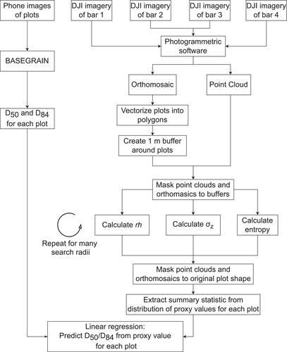
This study involved a field experiment along a river reach during which we collected UAV imagery and ground truth data. This field experiment was followed by processing these data with SfM photogrammetry and then performing statistical grain size analyses. This data processing workflow is represented in Figure 1.
2.1 Field experiment site description
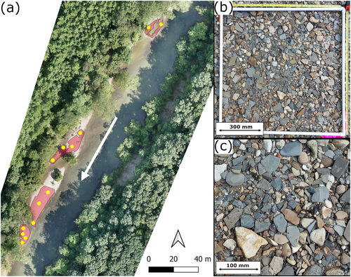
We conducted the experiment along a reach of the Olentangy River in Columbus, Ohio (Figure 2). The coordinates of this site are 40.133717°N, 83.032964°W. The length of our study reach is approximately 250-m long, and the bankfull width along this reach is approximately 50 m. The Olentangy River is a meandering stream with a gradient of approximately 0.001 and is classified as a Rosgen Type C stream. Our study reach is located within the Highbanks Metro Park, and the banks along this reach contain forests. We limited our study to a series of gravel bars along this reach, which is common for remote sensing assessments of grain size because of the impact of water refraction on image properties (Woodget & Austrums, 2017). These gravel bars consist of alluvial sands, gravels and cobbles. The bedrock at this location is the Ohio Shale, and colluvial shale fragments are present throughout the gravel bars because of erosion of the banks. The clasts in this reach are predominately platy. Discharge at this location is influenced by a dam that is approximately 30 km upstream. A stream gauging station maintained by the United States Geological Survey (USGS) is located near our study site.
We conducted our experiment in early September 2021 during a period of low flow. For the 2021 water year, the USGS stream gauge reported an annual mean discharge of 15.77 m3/s, and the minimum and maximum daily mean discharge were 0.920 and 134.5 m3/s. On the day of our survey, the mean daily discharge was 2.25 m3/s. This was within the 20th percentile of daily mean discharges for the 2021 water year. Weather conditions were clear and sunny. We initially performed a pebble count by traversing the gravel bars in a grid pattern and measuring each sample with a gravelometer. We sampled a total of 110 grains from across the four bars. The purpose of this pebble count was to act as a comparison to our remote sensing analysis.
2.2 Collection of calibration imagery
We collected calibration imagery over subaerially exposed grains. To do this, we constructed a 0.9 m × 0.9 m frame from polyvinyl chloride (PVC) pipe. We then selected locations throughout the gravel bar for calibration plots. These plots should ideally be homogenous in terms of grain size throughout each individual calibration frame, and together they should all represent a range of grain sizes. To ensure an even distribution of plots throughout the study area, we placed plots near the downstream edge of a bar, in the centre of a bar and near the upstream edge of a bar. We distributed a total of 13 calibration plots throughout the four bars in our study reach. This number of samples follows the findings from Vázquez-Tarrío et al. (2017) who used a sensitivity analysis to show that a minimum of 9 or 10 calibration plots are recommended for calibrating statistical grain size models. To collect calibration images, we placed this frame over a selected location. We then marked two opposite corners of the frame and geolocated these markers with a Trimble real-time kinematic (RTK) geographical positioning system (GPS) unit (Figure 2b). We took images of these plots with a smartphone camera consisting of a 64 MP Sony IMX682 sensor with a 35 mm equivalent focal length of 25.4 mm. These images had a resolution of 9248 × 6936 pixels. To take these images, we positioned the camera approximately parallel to the ground and held the camera at a height such that the calibration image fully captured the frame.
2.3 UAV survey
We manually flew a DJI Mavic 2 Pro at an altitude of approximately 4 m and took images throughout the gravel bars. This drone contains an integrated camera with a 20 MP (5472 × 3648 pixels) 1” CMOS sensor with a 35 mm equivalent focal length of 28 mm and a field of view of 77°. This drone uses a three-axis gimbal, which works to stabilise the camera and reduce blurriness in the collected imagery. While flying the UAV, we collected RGB images at nadir configuration and collected images that we visually estimated to have 70% overlap. Previous literature has shown that motion blur may negatively affect the quality of remote sensing-based grain size analysis (Woodget et al., 2018). To minimise the effect of motion blur, we flew at a low velocity and decelerated the drone when taking images. We separated the survey into four flights, and we collected a total of 427 images. The total area surveyed was approximately 700 m2, and it took approximately 1 h to complete the drone survey.
2.4 Ground truth data
The images of the plots that we took with a smartphone served as our ground truth data that would be used to calibrate and validate the statistical grain size models. The calibration frame served as a constant scale for the image so that the grains that were visible in the image could be measured. To estimate the grain size distributions within these plots, we used the photosieving software BASEGRAIN (Detert & Weitbrecht, 2013). We initially scaled each image according to the fixed size of the calibration frame. The average resolution of these photos was approximately 0.2 mm/pixel. The default software parameters tended to over-segment individual grains. To account for this, we adjusted the parameters to process the image more smoothly by decreasing medfiltsiz10 and increasing facgraythr1. After the photosieving process was completed, we post-processed the delineated grains by manually excluding non-grain objects (e.g., leaves and branches) and merging over-segmented grains. Previous work has shown that truncating the grain size distributions for the calibration data improves the performance of statistical grain size models (Vázquez-Tarrío et al., 2017). We truncated the grain size distribution at a minimum b-axis length of 10 mm, which is the default parameter for the programme.
2.5 SfM photogrammetry
We used Pix4Dmapper to process drone images and processed all of the images over each of the four flights as separate projects. Our GPS measurements served as ground control points for georeferencing the photogrammetric data. From the default calibration parameters, we changed the Internal Parameters Optimisation setting from ‘All’ to ‘All Prior’ to account for the flat and homogeneous nature of our imagery. For the point clouds, we selected a high point density. The resolution of the orthomosaics was set to be equal to the ground sampling distance of the imagery, which averaged approximately 0.8 mm/pixel among the separate flights. The georeferencing root mean square error (RMSE) for these projects ranged from 0.01 to 0.05 m. The average point densities of the point clouds were approximately 2.0 × 10⁷ points/m3.
We imported the processed point clouds and orthomosaics with our GPS measurements into CloudCompare and QGIS for further analysis. The point clouds were detrended to remove the effects of bed slope on our topographic analysis, which has been shown to influence results in previous literature (Brasington et al., 2012; Vázquez-Tarrío et al., 2017). For the purpose of testing calibration relationships between grain sizes and image and point cloud metrics, computing each combination of metric and kernel size throughout the entire study area would require too much computer storage and processing power, so we first crop the calibration plots from the orthomosaics and point clouds. To do this, we vectorised the calibration plots into polygons based on the geolocated corners of the plots. We then created 1-m buffers around each of these polygons. These buffers prevent edge effects from affecting the computation of the grain size proxies as using the original shape of the plots would lead the computation of metrics at points near the edges to become skewed towards the center of the calibration plot. The orthomosaics and point clouds were then masked by these buffers to isolate the calibration plots and the area surrounding them. After the computation of grain size proxies (discussed below), the resulting point clouds and images were clipped to the original shape of the plots.
2.6 Statistical grain size estimation
Using these clipped calibration plots, we computed three different point cloud and image metrics that have previously been used as proxies for grain sizes: roughness height (rh), the standard deviation (σ), and entropy. We computed all three of these metrics for both the point clouds and orthoimages. For each point or pixel in the point cloud and orthomosaic, these metrics, which serve as proxies for grain size, were calculated from the surrounding neighbourhood within a certain search radius or kernel size. Summary statistics based on the distribution of the metric values were then extracted from each calibration plot. Given the grain size percentiles obtained from the photosieving analysis and the statistical values for each grain size proxy, a statistical grain size model can be produced through linear regression.
The roughness height is a topography-based metric that corresponds to the deviation from the best-fitting plane of a neighbourhood of points in the point cloud (Chardon et al., 2020; Vázquez-Tarrío et al., 2017; Woodget et al., 2018; Woodget & Austrums, 2017). To compute this metric for the point cloud, we used the roughness tool provided by CloudCompare (CloudCompare 2.12, 2022). This tool permits various kernel sizes to be used, which define the radius of the neighbourhoods around each point. The result of this computation is a point cloud where each point contains a scalar value that is equal to its roughness height for a given kernel size. To transfer this metric to imagery, we implemented a similarly iterative procedure for each pixel whereby a plane is fitted to the greyscale values of the neighbouring pixels and the roughness height is calculated as the difference between the greyscale value for the pixel and the predicted greyscale value by the best-fitting plane.
The standard deviation of elevations, σZ, is a topography-based metric that has commonly been used in statistical grain size estimation (Groom et al., 2018; Heritage & Milan, 2009; Pearson et al., 2017; Vázquez-Tarrío et al., 2017). To calculate this metric, we used the KDTree class from SciPy, which is a scientific computing library for the Python programming language (Virtanen et al., 2020). We imported the point cloud and queried neighbouring points within a given radius using the functions from this class. For each point in the point cloud, we queried its neighbourhood, computed the standard deviation of the elevations within this neighbourhood and assigned this value to the respective point in the point cloud. To transfer this metric to imagery, we calculated the standard deviation of the greyscale values (σGrey) in the neighbourhood for each pixel.
2.7 Calibration and validation of grain size proxies
To determine the optimal radius or kernel size for these metrics, we used an iterative approach similar to the one presented by Woodget et al. (2018). For the topography-based metrics, we repeated the computations described above for kernel sizes ranging from 20 to 160 mm in a step size of 20 mm. For the image-based metric, we repeated the computation for kernel sizes ranging from 2 to 24 pixels in a step size of 2 pixels. Given the resolution of our orthomosaic, this translates to a range of kernel sizes from 1.6 to 16 mm.
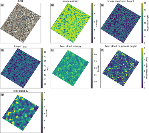
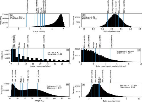
Figure 3 shows examples of the different grain size proxies for one of the calibration plots. In the image-based examples, lower proxy values correspond to larger grain. In the point cloud-based examples, higher proxy values generally correspond to larger grains. Figure 4 shows the corresponding distributions of values for the three metrics. For each distribution corresponding to the different combinations of possible kernel sizes and proxies, we extracted several summary statistics that relate to its location, spread and shape including the mean, different percentiles, standard deviation and skewness. To determine the statistic that best correlates with grain size variation throughout the calibration dataset, we expanded our iterative approach to test models calibrated on these different proxy distribution statistics.
We compared the performance of the different grain size proxies, kernel sizes and summary statistics through a leave-one-out cross-validation approach (LOOCV). One of the advantages of LOOCV is that it is a more robust method for model validation when using a small sample size such as ours. To do this, we first excluded one of the calibration plots from the dataset. The remaining plots were then used to calibrate a univariate linear regression model of the plots' grain size percentiles as a function of their proxy value statistic. We used this linear model to predict the grain size percentile of the plot that had been excluded from the calibration dataset. To repeat this for another plot, we excluded a different plot from the calibration dataset and calibrated a new linear model that was used to predict a grain size percentile for the excluded plot. This process was repeated until grain size percentiles for each plot had been predicted. The resulting validation relationship is a linear model between the observed grain size percentiles from the photosieving and the predicted grain size percentiles based on the LOOCV procedure. To quantify the quality of the validation result, we plot the observed grain size percentiles against the predicted grain size percentiles and compute the R2 and slope of the line of best fit. We repeated this LOOCV procedure for each of the summary statistics and three grain size proxies of interest over a range of kernel sizes.
3 RESULTS
The results of the ground truth data from the photosieving analysis and pebble count and the results of the statistical grain size estimation procedure are described below.
3.1 Ground truth data
Figure 5 shows the grain size distributions obtained through the Wolman pebble count and the photosieving analysis for the 13 calibration plots. Because of the use of a gravelometer, we focus only on the b-axis measurements obtained from photosieving for this analysis. In comparison to the Wolman pebble count, the photosieving distributions underestimate the frequency of small grains because of the truncation made at 10 mm.
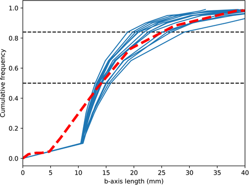
However, the range of D50 and D84 measurements obtained from the photosieving analysis includes the measurements made from the Wolman pebble count. We observed D50 measurements from 13.0 to 15.8 mm and D84 measurements from 18.9 to 29.1 mm throughout the 13 calibration plots. The D50 and D84 measurements from our pebble count were 14.1 and 25.1 mm, respectively.
3.2 Calibration and validation relationships
Figures 6-8 show how the slopes and R2 values of the validation relationships vary for the different summary statistics over the range of kernel sizes tested for each grain size proxy. For the imagery-based roughness height method, the models using the mean and different percentiles have been excluded (Figure 7). This is because of the low variance observed in these values among the 13 calibration plots as well as the discrete nature of the values producing erroneous models. For the imagery-based models, the use of the 10th percentile resulted in the best performance with the exception of D50 and D84 image roughness height models where skewness performed the best. The optimal kernel size for the imagery-based models ranged from 4 to 10 pixels. For the topography-based models, the use of the 10th percentile also resulted in the best performance with the exception of the D50 and D84 point cloud entropy models. The optimal kernel size for the topographic models ranged from 20 to 40 mm.
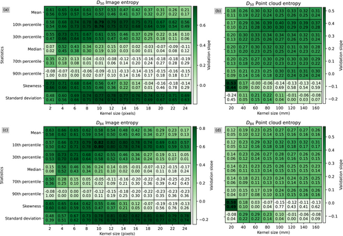
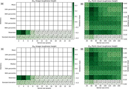
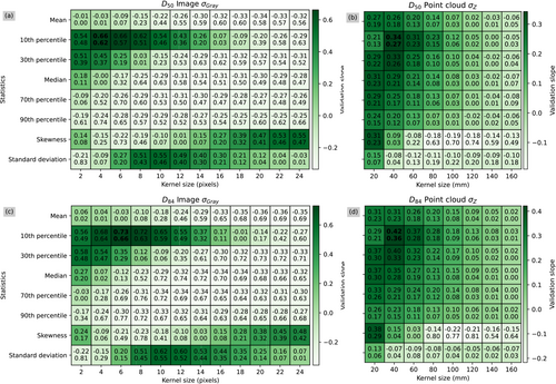
These figures demonstrate how the performance of these metrics relate to the kernel size used to process them. This kernel size represents the distance that most accurately captures the textural and roughness signatures that are present in the orthomosaics and point clouds. When the kernel size is too small, the grain size proxy becomes skewed by local deviations in texture or roughness so that the kernel window does not include an adequate number of grains to calculate a representative value for image texture or point cloud roughness. Conversely, when the kernel size is too large, the grain size proxy becomes less sensitive to textural and roughness variations, which causes the grain size proxy to inadequately detect textural and roughness features and have a weaker correlation with grain size.
Figures 9-14 show the calibration and validation relationships associated with the optimal combinations of proxy statistic and kernel size for each of the metrics applied to both the imagery and the topography. Out of these models, only two provide acceptable estimates of grain size: the image entropy model and the image σGrey model. The image entropy model performed best (Figure 9). The D50 model has a validation R2 of 0.76 and a validation slope of 0.79, and the D84 model has a validation R2 of 0.80 and a validation slope of 0.82. For the image σGrey metric, the D50 model has a validation R2 of 0.62 and a validation slope of 0.66, and the D84 model has a validation R2 of 0.66 and a validation slope of 0.73. Overall, all of these grain size models underestimate grain sizes, which are demonstrated by all of the validation slopes being less than one. This effect is least pronounced in the grain size models that use the image entropy and image σGrey metrics.
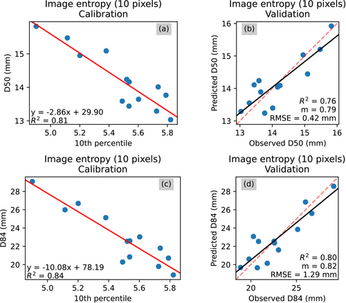
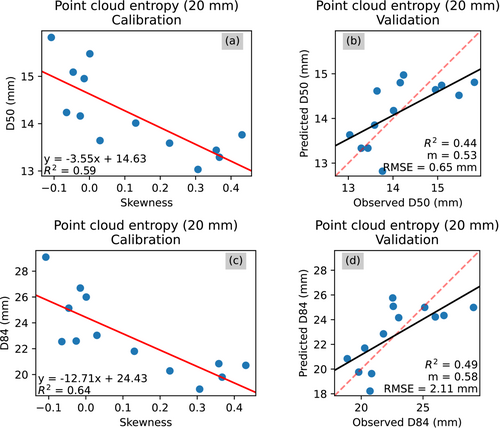
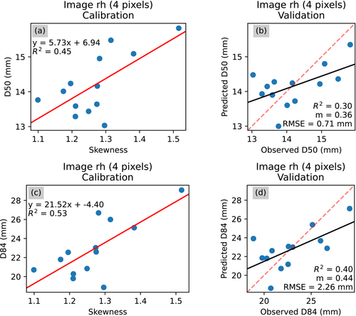
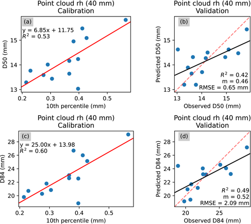
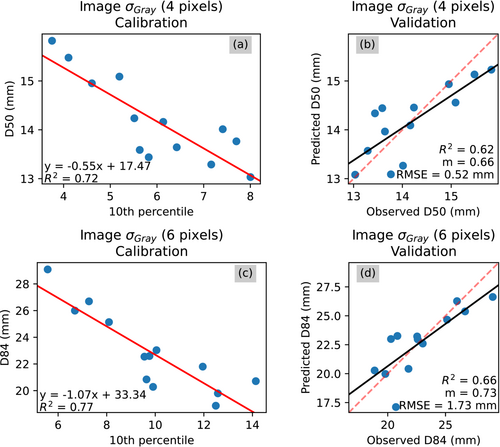
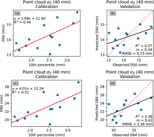
One general trend is that, for each grain size proxy, grain size estimates for D84 are better than those for D50 because the validation slopes and R2 values are slightly higher for the D84 models. However, the patterns of which models perform better and worse are the same regardless of the grain size percentile being predicted, and the ranking of how well each grain size metric performs is the same. Among both of the D50 and D84 models, image entropy is the best performing model and point cloud standard deviation is the worst.
The application of the entropy and standard deviation metrics to imagery results in superior performance than does the application of those metrics to topography. For the roughness height metric, the opposite pattern is observed and the application towards topography provides better grain size estimations than does the application towards imagery.
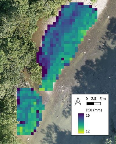
Figure 15 shows the application of the image-based entropy calibration model, which we found to be the best performing, to a subsection of the survey area. This demonstrates the ability for this grain size estimation method to detect patterns in grain size along fluvial gravel bars.
3.3 Outlier in calibration models
To understand the reason for why some of these grain size models may not perform as well as others, it is helpful to examine the worst performing one: the point cloud σZ model (Figure 14). The performance of this model is strongly influenced by an outlier that exhibits a high topographic signature yet small D50 and D84 measurements (Figure 14a and c). Calibration on the other plots through the LOOCV procedure results in an overestimation of the grain size for this plot (Figure 14b and d). This calibration plot has the smallest grain size out of all of the plots. Further analysis of the other models shows that this outlier is also present in the image roughness height (Figure 11) and point cloud roughness height (Figure 12) models. However, this plot is not as prominent of an outlier in the image entropy (Figure 9), point cloud entropy (Figure 10), and image σGrey (Figure 13) models.
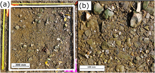
The grain texture of this outlier plot is shown in Figure 16. In comparison to the grain texture shown in Figure 2, which is more representative of the grain texture found throughout the study area, this plot contains a high amount of clay, and many of the grains are coated in clay from high flow events. Because of this, the surface color of the grains as well as the contrasts between grains might differ from the other plots. Additionally, while the grains shown in Figure 2 are mostly flat shales, there are several larger and more spherical grains distributed throughout this plot. This would have made the topographic signature of this plot higher than the others. This outlier contains grain texture that is unique from the remaining plots, so image-based and topography-based models computed using this plot may not perform well.
With respect to the standard deviation metrics, the better performance of the image σGrey model in comparison to the point cloud σZ model suggests that the image-based σGrey model is not as affected by this deviation in grain texture. Therefore, the topographic signature of this outlier plot is too different from the other plots such that it worsens the performance of the standard deviation model calibrated based on topography. For the roughness height metrics, both the image-based and point cloud-based models are affected by this outlier, which suggests that the roughness height metric is more sensitive to differences in topography and imagery. Conversely, for the entropy metrics, both the image-based and point cloud-based models show better fitting to this outlier. Therefore, in comparison to the other metrics, the entropy metric may be a more robust proxy for grain size when dealing with more heterogeneous calibration data.
4 DISCUSSION
In this section, we evaluate how effective the statistical grain size estimation techniques based on imagery compared to those based on topography. We follow this with a discussion of the strengths and weakness of our methodology.
4.1 Efficacy of image-based versus topography-based grain size proxies
Our results demonstrate that two image-based metrics computed from a UAV-derived orthomosaic performed better at estimating D50 and D84 measurements than topography-based metrics computed from UAV-derived point clouds. The calibration and validation R2 values for the image entropy and image σGrey models indicate a moderately good predictive relationship between image properties and the sedimentological characteristics of this river of interest that failed to be captured by the other metrics.
The poor performance of the topography-based metrics may be attributed to the characteristics of the grains within our study site such as their size, shape and degree of imbrication (Figure 17). Metrics for predicting grain size from topography have traditionally been applied in rivers where the grains are larger, which would make fine-scale topographic variations more significant (Woodget et al., 2018). The range of grain sizes studied in this paper is finer than previous UAV-based grain size estimation studies that have typically focussed on topography-based metrics. Smaller grains result in less significant fine-scale topographic variations between particles, which worsens the ability to correlate point cloud roughness to grain size. Additionally, a large portion of the grains within our study area are shales that are flatter in shape, which would result in very little fine-scale topographic variability near those grains. Furthermore, topography-based metrics have been shown to be sensitive to the imbrication of grains, where a high degree of imbrication limits the ability to use fine-scale topographic variations as a proxy for grain size (Casado et al., 2020; Heritage & Milan, 2009; Pearson et al., 2017). This is because imbricated grains are partially buried and angled such that they do not produce topographic signatures consistent with their size. We observed a slight degree of imbrication in grains throughout the study area (see Figures 2 and 16), which would have contributed to the poor performance of the topography-based metrics. Given the low flight height used in our UAV survey, the point clouds in our study have a high enough resolution where the effects of grain size might not be as important as those of grain shape and imbrication.
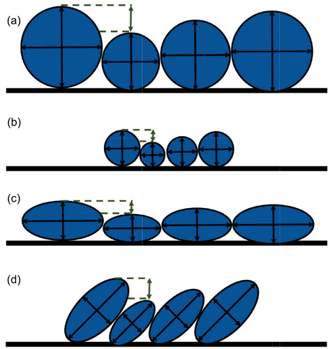
The image entropy and image σGrey metrics, which are computed from only a two-dimensional image of the grains rather than a three-dimensional point cloud, performed better than the topography-based metrics as it does not rely on the limited fine-scale topographic variability throughout our study area. Instead, these image-based metrics represent the textural characteristics of the orthomosaic, and our results show that these textural metrics correlate well with grain sizes. This finding agrees with previous work on grain size estimation through image texture. For example, Dugdale et al. (2010) suggested that entropy is a suitable metric for estimating smaller grain sizes as it amplifies the contrasts between grain boundaries through the logarithmic component in its computation. Because of this, entropy appears to be a more robust proxy for grain size in areas with smaller grains where the light–dark boundaries between particles tend to be less clear. The results of this study suggest that this behaviour of the entropy metric may extend to topographic properties of grains.
Recent research on techniques for grain size estimation from UAV imagery and SfM photogrammetry further supports our findings. For example, Woodget et al. (2018) similarly compared how image-based and topography-based metrics correlate to grain size, and they found that models calibrated on the roughness height metric yielded weaker validation relationships when compared to those calibrated on image entropy. Their study area had b-axis D84 measurements of approximately 0.07 m, whereas ours were approximately 0.025 m (Figures 9-14). Because we observe a similar contrast between the image-based and topography-based metrics, the results of this paper provide further evidence that image textural approaches are more accurate than topographic roughness approaches in settings where grain size, shape and imbrication limit topographic variability. Future research should attempt to clearly define the ranges in grain size, shape, and imbrication for which image textural metrics and topographic roughness metrics each perform optimally.
4.2 Recommendations and limitations
A graphical overview of the processes discussed in this paper is shown in Figure 1. This UAV-based workflow presented in this study has demonstrated promise at estimating grain size percentiles in rivers with inexpensive equipment. The statistical grain size models calibrated based on orthomosaic image texture were shown to perform best in this stream characterised by slightly imbricated medium-sized gravels. However, further research into the conditions that influence the performance of these metrics still needs to be carried out. This study demonstrates that processing both image-based and topography-based grain size proxies using UAV imagery is straightforward to translate into grain size estimates, and investigating a variety of kinds of grain size proxies when conducting UAV-based grain size estimation may prove to be a comprehensive method of quantifying grain size distributions in rivers.
A limitation to the methodology used in this study is the use of photosieving for the calibration data. Adams (1979) established that photosieving results in biased grain size measurements in comparison to standard sieve analyses. This is because photosieving measures only the two-dimensional appearance of grains in a horizontal plane whereas traditional methods incorporate measurements of the vertical dimension. Because of this, photosieving measurements may be inaccurate in areas where grains are partially buried or imbricated. (Butler et al., 2001; Graham et al., 2010; McEwan et al., 2000; Sime & Ferguson, 2003). While we compare the photosieving results to a Wolman count, this comparison may not be reliable given how few grains we sampled over a heterogeneous study area.
Our study examines how well different image and topographic metrics correlate with grain sizes obtained from photosieving. Because photosieving is also based on imagery, it is possible that the image-based models are inherently better at correlating with photosieving results than are the topography-based models. Both the photosieving and image-based metrics operate on the same two-dimensional horizontal plane, whereas the topography-based metrics are computed from vertical data that are perpendicular to that plane. Previous studies that used photosieving to calibrate topographic grain size models have demonstrated mixed success. Bertin and Friedrich (2016) used BASEGRAIN to measure grain sizes in patches of gravel bars with D50 values ranging from approximately 20 to 50 mm, and they noted that imbrication was present in their samples. Their correlation with σZ values obtained from SfM photogrammetry had a calibration R2 value of 0.96; however, their sample size was limited to three patches. Westoby et al. (2015) applied a similar methodology to patches of arctic moraines with D50 values between 8 and 20 mm. They correlated BASEGRAIN-derived D50 values to SfM-derived σZ values and reported a calibration R2 value of 0.225. In regards to image-based models, photosieving-based methodologies have been successful. Carbonneau et al. (2004) used photosieving to collect ground truth grain size data for their models based on image semivariance and reported a calibration R2 of 0.80. Their model contained patches with D50 values less than 160 mm. They noted that grains in their study area were weakly imbricated and discussed how this contributed to bias in their photosieving analysis and resulting grain size estimates. Dugdale et al. (2010) correlated entropy with D50 values obtained from field and aerial photosieving in an area with non-imbricated, loosely-sorted pebbles and cobbles. The D50 values ranged from 10 to 500 mm. They reported calibration R2 values between 0.69 and 0.84.
Previous literature show that the use of traditional field-based measurements to collect ground truth grain size data have often resulted in greater success for topography-based models. Brasington et al. (2012) analysed patches from different rivers that ranged from coarse rounder grains to finer platy ones. These patches had D50 values ranging from 10 to 120 mm. They found that D50 grain sizes obtained from pebble counts correlated well with σZ and reported a calibration R2 of 0.95. Vázquez-Tarrío et al. (2017) investigated non-imbricated gravels and cobbles within a braided river. Patches in this study had D50 values ranging from 20 to 70 mm. They used Wolman counts in their calibration plots and observed calibration R2 values of 0.89 and 0.66 for D50 models based on point cloud roughness height and σZ, respectively.
In studies that directly compare image-based and topography-based models, measurements of ground truth grain size data from imagery have not always led to image textural models outperforming topographic roughness ones. Woodget and Austrums (2017) manually measured the a- and b-axes of grains from imagery of calibration plots and reported that grain size models calibrated on point cloud roughness heights (R2 = 0.7987) performed better than those calibrated on image entropy (R2 = 0.4787). D84 values in these models ranged from 10 to 160 mm. Woodget et al. (2018) studied a gravel bar where grains were imbricated and patches D50 values between 20 and 100 mm. They also used manual measurements from imagery and found that point cloud roughness height models (R2 = 0.60) performed better than orthomosaic entropy models (R2 = 0.48). However, they ultimately concluded that models using their novel method based on single image texture outperformed both (R2 = 0.69). Despite this, the R2 values for the topography-based models in these studies are still notably worse than those reported by studies using traditional field-based methods. This suggests that measuring grains from imagery may not necessarily be suitable for collecting ground truth data when applying topography-based methods of grain size estimation. Therefore, to perform a fully comparable analysis on how well image textural and topographic roughness metrics can estimate grain sizes, traditional field-based methods other than photosieving should ideally be used to collect calibration grain size information.
One specific source of error that we observed in some of the image-based and topography-based models was the aforementioned outlier that produced a high topographic signature but a low grain size percentile measurement (Figure 16). The poor fitting of these models to this plot is because of the distinct characteristics of the sediment found within it. The higher clay content and more spherical grains in comparison to the other plots resulted in distinct signatures in the imagery and topography that several of the models were not able to resolve into a linear relationship like the image entropy and image σGrey were able to. The presence of fine sediments altered the surface colour, which would influence how strong contrasts between grains are in the image texture metrics. The heterogenous grain texture in this patch, which was characterised by differences in grain shape and imbrication, also contributed to deviations in its topographic signature. Beyond this, there are several factors that we expect to cause a patch to deviate from a linear relationship between grain size and image texture or topographic roughness. Differences in lighting will alter the textural signatures associated with grain boundaries. Additionally, the presence of non-grain features such as vegetation will cause topographic variations that are not associated with differences in grain size.
The limitations of photosieving might have further contributed to this outlier. Photosieving assumes that each grain lies flat on the surface such that the a- and b-axes are fully expressed from the images taken with a nadir perspective and that the c-axis is perpendicular to the surface. The microtopography near that particle is then controlled by the c-axis. When grains lie at an angle and are not flat, the photosieving measurements made from the nadir angle become smaller as the c-axis becomes visible and the expression of the longer a- and b-axes increases. This in turn allows the a- and b-axes to contribute more to the microtopography, inflating the computed metrics. As shown in Figure 16, there are many grains throughout this outlier plot that were oriented this way. This caused those grains to produce a high topographic signature in the point cloud but a small footprint in the nadir calibration imagery. Because of this, future efforts for statistical grain size estimation should attempt a variety of methods for measuring the calibration data set such as physical pebble counts in addition to photosieving. Such methods might be more appropriate for addressing heterogeneity in grain characteristics throughout a survey area.
One of the considerations that should be made when performing these statistical grain size estimation techniques is the choice of summary statistic that best represents the roughness or texture of each individual plot. This study showed that generally the skewness and the 10th percentile of the grain size proxy distribution correlated better with grain size variations than did the mean or median. Therefore, examining the use of different summary statistics may result in improved performance for this method of grain size estimation.
For the purpose of grain size estimation in rivers characterised by smaller grains, we showed that imagery-based approaches provide more accuracy than do topography-based ones. Therefore, image quality is vital for accurate sedimentological analyses in settings where grains may exhibit a limited degree of topographic variability. Our method of manually piloting the drone allowed us to limit blurriness in the captured images. Additionally, we limited our flight height to be much lower than the normal height used for most geomorphological surveys to maximise the resolution of our data. However, this method was slow and required multiple battery changes to fully cover the study area, which may prove to be problematic for larger and less accessible study areas. In the future, improving the battery life and the use of a higher resolution camera may expedite the image collection process. Future research to determine the optimal balance among image resolution, flight height and survey time will progress UAV-based grain size estimation techniques to be more accessible for river scientists. An additional concern for this methodology is the amount of fieldwork required to collect calibration data, and possible future research can possibly extract such calibration data from low-flying drone surveys.
5 CONCLUSION
We tested different methods of estimating grain size from UAV-based SfM photogrammetry over several gravel bars along a large meandering river in Ohio. The methodology presented in this paper demonstrates the ability of UAVs to provide a continuous estimation of D50 and D84 grain sizes for aerially exposed grains in a river reach. Statistical grain size models were calibrated on different image textural and topographic roughness metrics that were calculated based on UAV-derived orthomosaics and point clouds. Our study expands on previous work by analysing the use of different summary statistics for calibrating grain size models.
The overall patterns in grain size, shape and imbrication within this study reach weakened the applicability of topographic metrics in the grain size estimation models. This paper provides evidence that image textural metrics may provide more accurate grain size estimates in comparison to topographic roughness metrics when used in settings characterised by smaller, flatter grains; however, further work to clearly define the ranges where these metrics perform optimally still needs to be performed. These results have implications for grain size estimation methods beyond the statistically based ones presented in this paper, and it is likely that any other remote sensing techniques using imagery of grains will be more appropriate than topography-based approaches given grains with limited topographic signatures.
AUTHOR CONTRIBUTIONS
Tyler Wong: Conceptualisation; methodology; investigation; software; writing—initial draft; writing—reviewing and editing. Sami Khanal: Methodology; investigation; resources; writing—reviewing and editing. Kaiguang Zhao: Methodology; writing—reviewing and editing. Steve W. Lyon: Conceptualisation; funding acquisition; methodology; supervision; writing—reviewing and editing.
ACKNOWLEDGEMENTS
This work was partially funded through fellowships awarded by the Ohio State University Graduate School and the Ohio Agricultural Research and Development Center. Additional support came from the Swedish Research Council Formas under the grant number 2019-01094. Thank you to Shannon Pace, John Brett and Kushal KC for their assistance in the fieldwork for this project.
Open Research
DATA AVAILABILITY STATEMENT
The data used in this study are available from the corresponding author upon reasonable request.


