Semi-Quantitative Discrimination of Honey Adulterated with Cane Sugar Solution by an ETongue
Abstract
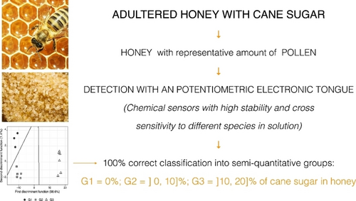
This study successfully applied a potentiometric E-tongue with 20 cross-selectivity lipidic polymeric membranes in the discrimination of three semi-quantitative groups, that represented the following intervals of honey adulteration percentage with cane sugar: 0 %; [0, 10]%; [10, 20]% of adulteration. We analysed five different types of Portuguese honey; five brands of cane sugar were added to the adulterated samples; a comparative analysis was then performed. Linear discriminant analysis coupled with a tabu search algorithm for feature selection was applied to the ETongue's analytical data to select the best model. A discriminant model with 12 sensors was obtained. This model classified correctly all samples in both in internal (train data, 15 samples) and external validation (test data,10 samples). Also, multiple linear regression with tabu search was applied to verify if ETongue's data would allow quantifying the honey's adulteration level. The results showed that it was possible to obtain a quantitative model but with unsatisfactory predictive performance in the test data group (external validation), giving, in general, values below the expected concentrations. E-tongue is a real-time green, flexible and low-cost analytical tool that requires minimum sample preparation and no special technical skills, being a promising tool for everyday application.
Graphical Abstract
1 Introduction
Honey is a natural sweetener produced by bees (Apis mellifera) and it can be classified in blossom honey (nectar of plants) or honeydew honey (secretions of living parts of plants or excretions of plant-sucking insects on plants).1 This food is mainly composed of sugars (glucose and fructose), water, and other constituents to a lesser extent, such as amino acids, enzymes, proteins, organic acids, carotenoids, vitamins, minerals, and aromatic substances.2 In addition, it is rich in flavonoids and phenolic acids that have several biological effects, for example, antimicrobial, anti-inflammatory and antioxidant properties.3
Honey's quality control is mandatory to allow its commercialization and to ensure its authenticity since it is prohibited to add or remove any ingredient.4 Due to its limited production and high market prices, honey is a product susceptible to adulteration.2, 5-7 Among the main ones, the following stand out: incorrect information of botanical (monofloral honey have the higher market value given the specificity of their aromas and flavors)5, 8 and geographic origin; the incorporation of water; the addition of sugar syrups, by adding to the bees′ diet or after honey production,9 for example: fructose corn syrup, corn sugar syrup, inverted sugar syrup and cane sugar syrup.10-12
The control of adulterants in honey is usually carried out by physico-chemical methods, such as hydroxymethylfurfural content, sucrose content, fructose/glucose ratio, and electrical conductivity.10, 13, 14 However, these parameters lack specificity, given the complexity of honey's composition which varies due to several factors such as climate, bee species, flora available, and bee feeding. For example, adulterating syrups have sugar profiles similar to honey, making it difficult to identify due to the fructose and glucose content.10, 14, 15
New instrumental methods have been applied in the study of adulterated honey, such as isotopic ratio mass spectrometry,16, 17 nuclear magnetic resonance spectroscopy,18, 19 high-performance liquid chromatography with electrochemical detection20 and diode-array,21 gas chromatography with ion mobility spectrometry detection9 and mass spectrometry22 and infrared spectroscopy.7, 23, 24 These techniques provide very detailed information about the compounds present in honey but are, in general, complex and time-consuming methodologies, with high cost, requiring controlled operational conditions and qualified operators for analysis.25 There are also studies using electrochemical multi-sensor systems, such as the electronic tongue (ETongue) and the electronic nose (ENose), in the identification of adulterants and food authenticity. Sousa et al.26 presented the application of a potentiometric ETongue to discriminate honey according to the floral origin. Indeed, Bougrini et al.25 were successful in determining the honey's country of origin, mono/polyfloral varieties and adulteration with glucose and sucrose syrup through a voltametric ETongue. Gan et al.5 used a potentiometric ETongue, ENose, and near-infrared to recognize botanical origin and adulteration by rice and corn syrup, having Etongue given better results in the adulteration study.
This work aimed to evaluate the performance of a laboratory-made potentiometric ETongue, together with chemometric tools of discrimination and regression, to detect/quantify adulterations of natural honey with cane sugar syrups. It was intended to select the best predictive models, using the Tabu search metaheuristic algorithm.
2 Materials and Methods
2.1. Materials and Reagents
For ETongue array construction, all reagents were from Fluka (minimum purity of 97 %; Sigma Aldrich, Switzerland): plasticizers (2-nitrophenyl-octylether, tris(2-ethylhexyl) phosphate, bis(1-butylpentyl) adipate, dibutyl sebacate, bis(2-ethylhexyl) phthalate); additives (octadecylamine, oleyl alcohol, methyltrioctylammonium chloride and oleic acid); supporting polymer (high molecular weight polyvinyl chloride). The tetrahydrofuran was from Sigma Aldrich (solvent produced in USA). Type II deionized water (AST 20, Portugal; conductivity lower than 1 μS/cm) was used in all assays, except for pollen analysis, where distilled water (automatic water distiller Kottermann 1033, Germany) was applied.
2.2. Sample Collection and Analysis
In this work, five different honey samples (identified as H1 to H5 samples) were acquired on a commercial surface, being from different beekeepers and geographical origins (respectively: Bragança, Portugal; Penacova, Portugal; Lousã, Portugal; Penacova, Portugal; León, Spain). The samples were stored in a dark environment at room temperature.
The melissopalynology analysis of honey was performed in a solution prepared with 10 g of honey dissolved in 30 mL of distilled water. After pollen extraction, by centrifugation, and chemical treatment according to the method reported by Louveaux et al.,27 the pollen grains were stained using a fuchsin solution (Merck) mixed with glycerin (Absolve). Pollen identification and count were carried out using an optic microscope (Leitz Messtechnik GmbH, Wetzlar, Germany) with 400× and 1000× objectives (the last one was used when greater detail was required for pollen identification). For each honey sample, a minimum of 1000 grains of pollen was counted, and in case of doubt, the analysis was repeated. Reference standards obtained from Portugal honey flora (available at Instituto Politécnico de Bragança, Portugal) were used for grain pollen identification and the samples were classified based on their floral origin according to their found pollen morphology. In general, a honey sample can be classified as Lavandula monofloral honey if its Lavandula pollen content is higher than 15 %, Castanea monofloral honey if its pollen is higher than 90 % and monofloral honey of other pollens if its respective pollen content is higher than 45 %.28, 29
The honey's color was measured in solutions of 5 g of honey dissolved in 10 mL of water, at 635 nm (UV/Vis spectrophotometer, Jenway, Genova model), using a quantitative millimeter Pfund (mm Pfund) scale,30 according to the equation: mm Pfund=−3870+37,139× Absorbance. The quantitative mm Pfund scale considers 7 levels of color for honey:31 water white (8< mm Pfund), extra white (8< mm Pfund ≤17), white (17< mm Pfund ≤34), extra light amber (34< mm Pfund ≤50), light amber (50 mm Pfund ≤85), amber (85< mm Pfund ≤114) and dark amber (>114 mm Pfund).
Also, five samples of cane sugar from different brands and colors (identified as C1 to C5 samples) were purchased. These colors were selected so that when adulterating the honey samples, the original color of the honey did not change.
2.3. Adulterated Samples
Solutions of the different cane sugars were prepared by dissolving 16.3±0.3 g into 100.0 g of water, which assured to obtain an average Brix% value of 13.6±0.1 %, same value as that obtained in natural honey samples.
The honey solutions were prepared by mass measurement of the natural honey and cane sugar solutions, to obtain three semi-quantitative groups of a percentage of adulteration: 0 %; [0, 10]%; [10, 20]%. Table 1 identifies the honey and cane sugar samples used in the preparation of the solutions and shows the values of honey's percentage of adulteration, as well as the respective semi-quantitative groups.
Solution |
Mix ID |
Adulteration% |
Group |
|---|---|---|---|
1 |
H1 |
0 |
G1 |
2 |
H1+C1 |
2.2 |
G2 |
3 |
H1+C1 |
5.0 |
G2 |
4 |
H1+C1 |
10.1 |
G3 |
5 |
H1+C1 |
20.0 |
G3 |
6 |
H2 |
0 |
G1 |
7 |
H2+C2 |
6.7 |
G2 |
8 |
H2+C2 |
10.8 |
G3 |
9 |
H2+C2 |
13.6 |
G3 |
10 |
H2+C2 |
16.2 |
G3 |
11 |
H3 |
0 |
G1 |
12 |
H3+C3 |
3.8 |
G2 |
13 |
H3+C3 |
5.8 |
G2 |
14 |
H3+C3 |
8.6 |
G2 |
15 |
H3+C3 |
11.9 |
G3 |
16 |
H4 |
0 |
G1 |
17 |
H4+C4 |
4.8 |
G2 |
18 |
H4+C4 |
10.0 |
G2 |
19 |
H4+C4 |
14.8 |
G3 |
20 |
H4+C4 |
19.7 |
G3 |
21 |
H5 |
0 |
G1 |
22 |
H5+C5 |
4.5 |
G2 |
23 |
H5+C5 |
9.6 |
G2 |
24 |
H5+C5 |
14.2 |
G3 |
25 |
H5+C5 |
19.6 |
G3 |
- H – honey; C – cane sugar; G1: 0 % of adulteration; G2: [0, 10]% of adulteration; G3: [10, 20]% of adulteration.
All solutions were prepared with volumes higher than 70 mL for ETongue analysis.
The adulterated samples (honey plus sugary solutions) were analysed using mid-infrared analysis, as described by Kelly et al.32 For analysis with ETongue, the honey solutions were prepared by measuring 10.0 g of honey into 50.0 g of water. The Brix% of the five natural honey solutions were measured by a Digital Handheld Refractometer (Brix%: 0–50 %; VWR ATC) and presented an average value of 13.6±0.1 %.
2.4. Potentiometric ETongue Device
The potentiometric ETongue was an all-solid multi-sensor device that included 20 sensors prepared with polymeric membranes obtained by mixing 32 % of polyvinyl chloride as polymeric matrix, 65 % of one plasticizer compound (A: 2-nitrophenyl-octylether; B: tris(2-ethylhexyl) phosphate; C: bis(1-butylpentyl) adipate; D: dibutyl sebacate; E: bis(2-ethylhexyl) phthalate) and 23 % of one membrane additive (1: octadecylamine; 2: oleyl alcohol; 3: methyltrioctylammonium chloride; 4: oleic acid). According to these codes, the sensor B2 has a polymeric membrane with plasticizer B (tris(2-ethylhexyl) phosphate) and addictive 1 (octadecylamine). The additive compounds have a long carbon chain with different functional groups, being non-specific, presenting low selectivity, and cross-sensitivity to the different species in the samples (both inorganic and organic, ionic, and non-ionic).33, 34
The multi-sensor device was built in a cylindrical piece of acrylic with an architecture already described in previous work.35 This device together with a double junction Ag/AgCl reference electrode was connected to a multiplexer Agilent Data Acquisition/Switch Unit model 34970A, which was controlled by the Agilent BenchLink Data Logger software, installed in a computer, for the sensor signals acquisition.
ETongue analysis of each solution was performed after a period of stabilization of 3 min, after which the 20-signal profile was obtained. Between sample analysis, the system was washed with deionized water and cleaned with absorbent paper.
2.5. Statistical Analysis
All data were analysed using the statistics program R, version 3.2.0 (The R Foundation for Statistical Computing, Vienna, Austria). The R statistical packages caret,36 ggplot2,37 MASS,38 MVN,39 PerformanceAnalytics,40 tabuSearch41 were used.
An independent data matrix of 25 lines (solutions) and 20 columns (sensors) was obtained from the ETongue analysis to the 25 prepared solutions (Table 1). The dependent variable corresponded to the group's identification to which each solution belonged. The multivariate discrimination model was obtained considering the 15 initial solutions as train data (prepared with 3 honey samples), having also allowed performing internal validation, and the remaining 10 solutions (prepared with 2 honey samples, not included in the train data) as test data, to validate the model obtained in its prediction capability. Each sensor in train data was centered (subtract mean from values) and scaled (divide values by standard deviation) and, using the same procedure, the test data.
Linear discriminant analysis (LDA) was the selected supervised learning technique to differentiate between natural and adulterated honey samples, considering the three semi-quantitative groups.
Tabu Search (TS), a metaheuristic feature selection algorithm, was applied to select the best subset of sensors to use at LDA. Feature selection allows a reduction of the dimensionality of the study allowing to remove redundant, irrelevant, or noisy data, improving predictability. The TS algorithm is a local search procedure that allows the exploration of the solution space beyond local optimality. It incorporates adaptive memory that allows the implementation of procedures that are capable of searching the solution space effectively since it acts both as a local and global search method. The information collected during the search is used to guide the responsive exploration,42 by identifying a subset of moves that are feasible to improvements and also to establish prohibitions (tabu) to prevent the search from coming back to previously-visited solutions.43 Overall, this search technique permits strong local search performance but with dependence on the initial solution and serial iterative search process.44 The algorithm was applied by defining the arguments to 50 iterations in the preliminary search of the algorithm; 5 as a tabu list size; 4 as the maximum number of restarts in the intensification stage of the algorithm; and, 20 as the number of neighbor configurations checked at each iteration.41
The model's performance was evaluated with internal validation by applying cross-validation with k-folds. In this work, 9 folds were used, which implies evaluating the discriminatory performance of 9 different models. As evaluation criteria of cross-validation, the average value of accuracy, representing the proportion of correctly classified observations obtained from the 9 LDA models, was used.
Of all the obtained models, the best model was selected and evaluated on their predictive power in the train and test data, by using the global results of accuracy, as well as those of sensitivity and specificity, which are commonly used to measure the performance of a predictive classification model.45
Sensitivity (True Positive Rate, TPR) is the proportion of identified positives in each group:45 Sensitivity=True Positives/(True Positives+False Negatives).
Specificity (True Negative Rate, TNR) is the proportion of identified negatives in each group:45 Specificity=True Negatives/(True Negatives+False Negatives).
To verify the LDA assumptions,46 data is tested if have: multivariate normal distribution; same within-group variance-covariance structure for all groups (groups have equal dispersions); multicollinearity (requires that no discriminating variable be perfectly correlated with another variable); and presence of outliers.
Multiple linear regression (MLR) together with TS, for feature selection, was applied to verify if the signal profiles allowed to obtain a prediction quantitative model of the adulteration levels in honey solutions. The best model was selected considering the predictive ability towards the train and test data. The model's performance was evaluated by using 9 folds cross-validation (gives 9 model attempts) to evaluate de predictive ability to new data by internal validation (train data), using the average of root mean square error (RMSE) and determination coefficient (R2). To visualize and evaluate the ETongue capability to quantify the levels of adulteration of honey with cane sugar solution, a simple linear regression model was established between the predicted MLR-TS model and real values for train and test data groups. The results were considered satisfactory if the linear regression parameters were close to the theoretical values:47-49 ‘zero’ (0) for root square error (RSE) and intercept; ‘one’ (1) for slope and the determination coefficient.
3 Results and Discussion
3.1. Samples
Table 2 presents the results from pollen and color analysis of the five honey samples. Only samples H2 and H5 have the main pollen (Echium spp and Erica spp, respectively); with predominance above 45 %, these samples according to what is reported in the literature are classified as monofloral honey50 (viper honey and heather honey, respectively). In general, when the pollen spectrum contains more than 45 % pollen of the same species, the so-called dominant species, the honey is classified as monofloral.51 The honey's color varied between clear amber and dark amber, being expected that the chemical composition would also vary.
Sample |
Two main pollens |
Type |
mm Pfund |
Color |
|---|---|---|---|---|
H1 |
41.7 % Castanea spp; 14.0 % Leontondon spp |
Multifloral |
59.3 |
Clear amber |
H2 |
53.4 % Echium spp; 12.3 % Erica spp |
Monofloral |
88.7 |
Amber |
H3 |
32.9 % Morus spp; 26.3 % Cistus spp |
Multifloral |
171.9 |
Dark amber |
H4 |
35.3 % Castanea spp; 10.4 % Lavandula spp |
Multifloral |
67.5 |
Clear amber |
H5 |
52.2 % Erica spp; 27.9 % Trifolium spp |
Monofloral |
137.7 |
Dark amber |
The five samples of unrefined cane sugar (identified as C1 to C5 samples) presents the following label descriptions: C1 - light yellow; C2 – brown; C3 – intense brown; C4 – intense yellow; C5 – golden yellow. As previously referred, the honey and cane sugar pairing was defined so that when adulterating the honey, its color was not changed.
Overall, the purpose of using different samples of honey and cane sugar was to guarantee high variability within the solutions to be analyzed with the ETongue.
3.2. Potentiometric ETongue Analysis
ETongue analysis was carried out in 3 min due to the sensors’ stability, considering that in the next 5 min the sensors had high signal stability over time, as shown by the variation of the signals from the 20 sensors from 3 to 8 min, which presented %RSD <0.7 % (results obtained for the adulterated honey solution number 23). Globally, the 20 sensors revealed signal variations in the analysis of the 25 honey solutions from 17 to 47 mV, meaning that the sensors had a sensitivity to the variability within the analyzed solutions.
Figure 1 depicts the potentiometric signals of all 20 sensors for the five honey samples. The sample H4 showed a different profile, which demonstrates that the honey matrix is characterized by the global contribution of the floral origin, which can be evaluated by the composition of non-predominant pollens (Table 2 shows the second most predominant pollen to highlight the differences between honey samples with the same predominant pollen). The figure also shows that although it is possible to differentiate the remaining 4 samples, the H3 and H5 samples, as well as the H1 and H2 samples have great similarities in the sensor profile. The variability in the profiles of potentiometric signals between the five honey samples was not avoided and, therefore, was present in the division of the data in a training and test group for the multivariate study of discrimination between kinds of honey without and with adulteration of cane sugar.
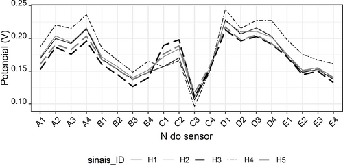
ETongue's signal profile of each honey sample.
3.3. Linear Discrimination Analysis with Tabu Search
The 15 initial solutions described in Table 1 were used as train data and the rest, as test data. The train data was standardized, the sensor's columns were centered and scaled, being the obtained arguments also applied to the test data.
The LDA-TS was applied to select the best LDA model using the best subset of sensors for discriminating the honey samples that were adulterated with cane sugars from the natural honey samples. The search considered all sensor subsets possibilities (1 to 20 sensors) and it allowed to solve model fitting by criteria maximization: train accuracy and test accuracy. The TS algorithm was applied to a total number of 150 iterations, with a number of 50 iterations at each preliminary search and 20 neighbors visited at each iteration. Figure 2A depicts the overall sensor subsets used to evaluate the best LDA model and Figure 2B, the number of times each sensor was used in the Tabu search iterative process. These figures show how the TS iterations were carried out, and the variables that seemed to be included in almost every iteration (most important). The six most used sensors in the TS iterations, in descending order, were: B3; A1; B4; B2; A3; and E4.
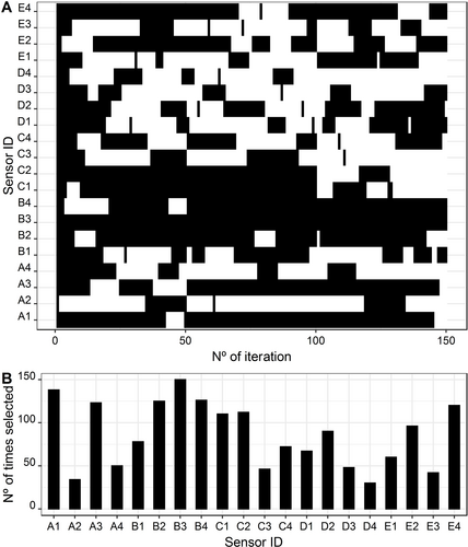
Linear discriminant analysis: A) Subset of selected sensors in each iteration; B) Number of times each sensor was used in the Tabu search iterative process.
The 9 folds cross-validation obtained an average value of accuracy of 0.3±0.4, which is representative that some of the samples are very important in the adjustment of the model, such as natural honey solutions (group G1), with the presence of only 3 samples, implying that their removal from the model adjustment would significantly change the percentage of correct classifications. This situation may be attributed to the fact that in the G1 group there are few samples of natural honey, compared to the representation in the remaining two groups (each with six samples).
The selected best model had 12 sensors: A1, A3, B2, B3, B4, C1, C2, C4, D2, E1, E2, and E4. This subset included all the 6 sensors most used in the TS. In this work, the polymeric membranes with the plasticizer D were the least represented in the LDA-TS model to discriminate between natural honey and adulterated honey samples. The obtained LDA-TS model has two discriminant functions that represent 100 % of total data variability, being the contribution of the first function of 98.6 %. In this model, the most relevant sensors were E2 and D3. Figure 3 shows the LDA plot representing the train data in the bi-dimensional space defined by the two discriminant functions and the grouping boundaries lines.
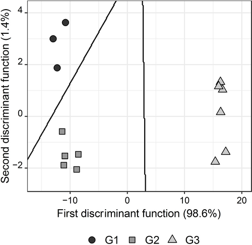
Honeys′ discrimination (2D plot of the first 2 discriminant functions and respective class membership boundaries). G1=0 %; G2=[0, 10]%; G3=[10, 20]% of honey adulteration degree with cane sugar.
This model allowed us to have 100 % of correct classifications, using both the train data and test data. Therefore, the sensitivity and specificity in each group were 100 %. These results showed the effectiveness of ETongue to distinguish naive honey samples from adulterated ones. It should be emphasized that the experimental design did not facilitate the application of LDA because, in the training data, the groups did not present the same sample sizes; as can be seen in Table 1, the group G1 was the least represented in training data, with only 3 solutions. Considering the global results obtained, it is expected that the discriminant model may be improved if there is greater representability of natural honey, ensuring variability, in training data.
3.4. LDA Assumptions
The performance of a predictive LDA model depends on the data meeting the assumptions but, evidence that certain of these assumptions can be violated moderately without large changes in incorrect classification results. Mainly, if it is used a larger sample size, the more robust the analysis is to violations of these assumptions. The homogeneity of multivariate dispersions was confirmed by using Bartlett (test for data that is normally distributed; p-value=1) and Fligner-Killeen (a non-parametric test which is very robust against departures from normality; p-value=1) tests, which are tests of group's homogeneity of variances. The multivariate normality of the independent variables (sensors) was confirmed by the Doornik-Hansen's test (p-value=0.80). Regarding the presence of outliers, their detection was done by visualizing the extreme values (outliers) in the box plot of the independent data (Figure 4). As can be seen, the three extreme values (solution 4) belonging to sensors E1, E2, and E4 are marked, which were not considered outliers (due to not having been repeated in the other sensors) but only specific results from these sensors associated with the matrix of that sample.
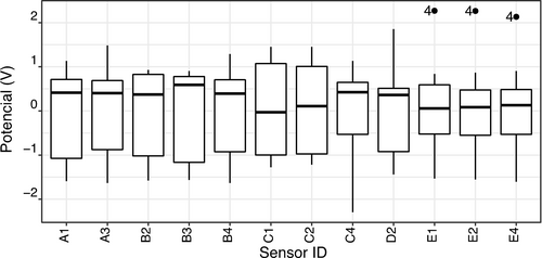
Boxplot of the potentiometric sensor's signals (independent data, centered and scaled) used in the LDA-TS model.
Considering that the analysis was carried out with an ETongue with cross-sensitivity polymeric membranes, multicollinearity was also expected between the sensors. In the sensor subset selected by the TS algorithm, the correlations between the signals’ sensors for the training data varied between 0.59 and 0.992. However, it is reported that the LDA technique is robust to a certain degree of these assumptions52 and that although the assumptions are important, the model's robustness is confirmed with its ability to predict new samples (test data).
3.5. Multiple Linear Regression with Tabu Search
In order to assess whether the signal profiles allowed to obtain a quantitative model to predict the honey's adulteration level with sugar cane solution, MLR-TS was applied to the training data used, in the LDA-TS section, and then verified the predictive ability of the selected model in the test group data. The signal profiles were also standardized (centered and scaled). The quantitative adulteration levels (Table 1) ranged between 0 and 20 %.
The conditions applied to the TS algorithm used a total number of 200 iterations, with a number of 50 iterations at each preliminary search and 20 neighbors visited at each iteration. Figure 5A shows the overall sensor subsets used to evaluate the best MLR model and Figure 5B, the number of times each sensor was used in the Tabu search iterative process. As referred previously, these figures show the TS iterations performed and the variables that seem to be included in almost every iteration. The six most used sensors in the MLR-TS iterations, in descending order, were: A1; C2; B4; B2; B3; and, C1. Comparing Figure 2B and 4B, it appears that the sensors have similar representability in the TS iterations.
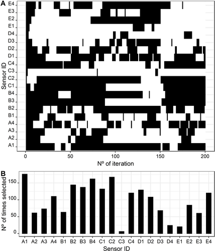
Multiple linear regression: A) Subset of selected sensors in each iteration; B) Number of times each sensor was used in the Tabu search iterative process.
It should be referred that it was possible to obtain several MLR-TS models having fittings with determination coefficients higher than 0.990, but without satisfactory ability to predict the adulteration levels present in the test group data (determination coefficients equal or lower than 0.76). The selected best model presented below highlights this situation. It has 12 sensors, including the 4 sensors most used in the TS: A1, A3, B1, B2, B3, B4, C1, C2, D2, E2, E3, and E4. Only the sensors B1 and E3 were not included in the best LDA-TS model presented in a previous section, inferring that quantitative information was used in the discrimination of the three defined groups.
The overall results of RMSE and R2 on the cross-validation study showed that, as also referred to in the LDA-TS section, some of the samples are very important in the adjustment of the model, implying that their removal from the model adjustment significantly changes the model's MLR-TS quality.
The best MLR-TS model presented a RSE value of 1.41 and a R2 value of 0.992. The linear relation between the MLR-TS model predicted and expected adulteration values for train data showed a slope and R2 of 0.997 (intercept equal to zero statistically since, not significant at the level of 5 %), as well as a low residual standard error of 0.53.
For the test group data, the results for all the linear relation between the predicted and expected values were not satisfactory: the linear equation obtained had no significant intercept, at the level of 5 %, and was set to zero; slope has the value of 0.69±0.13, with a confidence interval ([0.40, 0.98] at the significance level of 5 %) that did not include the theoretical value (unity); RSE value was equal to 4.92 and R2 value equal to 0.76.
Figure 6 presents these linear comparisons between the predicted values by the MLR analysis versus actual values of the honey's adulteration levels, for the train and test groups. It shows a good fit for the train data but not for the test data, where it was found that 5 of the samples are quite far from the expected values, contributing to an adjustment with slope and R2 values quite far from the theoretical value (unity). These results showed that the quantitative information within the signal's profile was not enough to obtain a robust MLR model for the quantitative prediction of the adulteration levels of sugar cane in the honey.
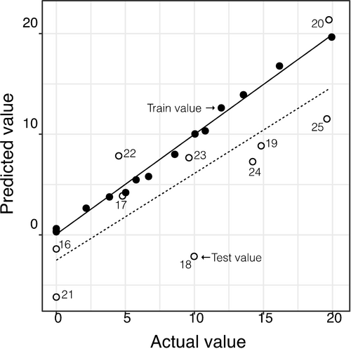
Quantification of honey's adulteration levels using a potentiometric ETongue
The possibility to be able to quantify the honey's adulteration levels is not discarded if: more natural and adulterated honey samples are included in the study to achieve greater representability of variability in the samples and therefore, a better quantitative model training; other non-specific and cross-sensitive lipid polymeric electrodes with analytical responses that improve quantitative analytical responses. The possibility of adjusting the sample matrices is also not ruled out, that is, making samples similar by adding, for instance, a total ionic strength adjustment buffer, important for potentiometric measurements. The objective would be to verify if it is possible to reduce the matrix effect of the honeys in the quantification model and, simultaneously, to increase the differences between them.
However, with regard to the cross-sensitivity sensors, the results showed the adaptability of the electronic tongue to the present study, which was expected considering that these polymeric membranes have already shown good performance in discrimination studies. For example, the identification of goat milk adulteration with bovine milk,33 gliadins semi-quantitative detection in foodstuffs,53 discrimination of monofloral honey samples with a broad pollen profile,26 and honey pollen profile assessment.54 There are also quantitative sugar works with the sensors used, for example, the work of Arca et al.49 that carried out sugars’ quantification (glucose, fructose, and sucrose) in standard solutions, Dias et al.55 that quantified, accurately, healthy and sensory indexes (glycemic load, fructose intolerance index, sweetness perception, total acid flavor, and well-balanced flavor) in beverages and Dias et al.,56 which performed a semi-quantitative and quantitative analysis of sugars (fructose and glucose) in soft drinks.
Also, the overall results were in accordance with the other works5, 25 that showed the ETongues’ efficacy (voltametric and potentiometric, respectively) in discriminating adulterated honey.
4 Conclusions
A potentiometric ETongue was applied successfully in the study of honey samples adulterated with cane sugar solutions. This fast multi-sensor system (non-specific lipid polymeric membranes coupled with LDA and TS variable selection algorithm) had a very good predictive performance to identify adulterated honey samples, being a powerful tool for quality control. Although the quantitative analysis showed sample matrix's effects, in the future, it is expected to use a total ionic strength adjustment buffer that could allow solving this relevant issue, which could also increase the range of Etongue applications.
This tool may be used as a triage prior traditional analytical methods considering its low-cost, simple measurement process, minimal sample pre-processing, adaptability to a complex matrix and compatible with green analytical chemistry.
Author Contribution Statement
ETongue analysis, writing – review and editing, statistical analysis – Luís G. Dias; writing – review and editing, statistical analysis - Evandro Bona; review and editing, pollinic and color analysis – Leticia M. Estevinho; state of art, writing – original draft preparation, data treatment – Master students (Andressa R.S. Bruni, Camilla P. Anizelli, Marcela Zangirolami and Patrícia C. Lima). All authors have read and agreed to the published version of the manuscript.
Acknowledgements
This work was carried out in the course of ‘Electronic Tongue and Nose in Food Technology’ of the Master's degree in Food Technology of Universidade Tecnológica Federal do Paraná, Campo Mourão, Brasil. This study was financed in part by Conselho Nacional de Pesquisa e Desenvolvimento Tecnológico (CNPq, 308153/2018-9) and the Coordenação de Aperfeiçoamento de Pessoal de Nível Superior - Brasil (CAPES) – Finance Code 001. The Portuguese authors are grateful to the Foundation for Science and Technology (FCT, Portugal) for the financial support through national funds FCT/MCTES (PIDDAC) to CIMO (UIDB/00690/2020 and UIDP/00690/2020) and SusTEC (LA/P/0007/2021).
Conflict of interest
Luís G Dias declares that he has no conflict of interest. Camilla P Anizelli declares that she has no conflict of interest. Patrícia C Lima declares that she has no conflict of interest. Evandro Bona declares that he has no conflict of interest. Informed Consent: Informed consent was obtained from all individual participants included in the study. Ethical Approval: This article does not contain any studies with human participants or animals performed by any of the authors.
Open Research
Data Availability Statement
The data that support the findings of this study are available from the corresponding author upon reasonable request.


