Pure Isotropic Proton NMR Spectra in Solids using Deep Learning
Graphical Abstract
Abstract
The resolution of proton solid-state NMR spectra is usually limited by broadening arising from dipolar interactions between spins. Magic-angle spinning alleviates this broadening by inducing coherent averaging. However, even the highest spinning rates experimentally accessible today are not able to completely remove dipolar interactions. Here, we introduce a deep learning approach to determine pure isotropic proton spectra from a two-dimensional set of magic-angle spinning spectra acquired at different spinning rates. Applying the model to 8 organic solids yields high-resolution 1H solid-state NMR spectra with isotropic linewidths in the 50–400 Hz range.
Introduction
The resolution of 1H solid-state NMR spectra is limited by broadening due to the homonuclear dipolar interactions between the abundant 1H spins.1 Magic angle spinning (MAS)2 helps reduce dipolar broadening by spinning the sample around an axis tilted at 54.74° from the direction of the main magnetic field. This process induces coherent averaging of second-rank tensor interactions such as the homonuclear dipolar interaction while having no effect on isotropic interactions such as the chemical shift. However, these interactions cannot be completely removed even at the highest spinning rates currently available. This results in residual broadening typically on the order of hundreds of hertz,3 which undermines the information contained in 1H solid-state NMR spectra.
In the CRAMPS approach,4 pulse sequences designed to remove homonuclear dipolar couplings can be combined with low or fast MAS to produce extra narrowing.5 At 100 kHz the linewidths obtained with MAS alone are about the same as the best results from state-of-the-art CRAMPS at slower MAS rates, and so far CRAMPS schemes have yielded no significant improvement for MAS rates above 65 kHz.
An alternate approach to achieving 1H homonuclear decoupling at fast MAS that does not rely on multiple-pulse averaging sequences6 is based on the anti-z-COSY experiment7 which exploits a simple 2D scheme that yields correlations between remote transitions of the coupling partners, and which removes the non-refocusable part of the residual dipolar broadening.6 This approach can typically provide a factor two reduction in linewidth compared to MAS alone, but contributions due to refocusable interactions will remain.
The dependence of residual splittings and shifts on the MAS rate  has previously been described as polynomial with respect to the inverse of the MAS rate, typically dominated by first- and, to a lesser extent, second-order terms.3, 8 In this light, Moutzouri et al. recently introduced a two-dimensional approach to obtain the pure isotropic (infinite MAS rate) spectrum of a solid from a set of spectra measured at different MAS rates.9
To process these two-dimensional datasets, they used a method of fitting an amplitude vector (i.e., the isotropic spectrum), together with parametric broadenings and shifts, to reproduce the set of 1H spectra acquired at varying MAS rates by convoluting the MAS-independent amplitude vector with the MAS-dependent shift and broadening function. While this provides a powerful method to obtain isotropic spectra, several assumptions and restrictions inherent to this fitting approach may limit its performance.
Deep learning (DL) has tremendously improved many areas of science and technology over the last decade, thanks to the ability of deep neural networks (NNs) to learn complex functions in an automated manner.11 In particular, convolutional neural networks (CNNs) are popular models to extract information from images or spectral data12 and have been used in the context of NMR to denoise or deconvolute spectra, to reconstruct under-sampled spectra, to virtually decouple spectra, and to perform automated peak picking.13
Recurrent neural networks (RNNs) are a class of neural network developed to process time series data. The “long short-term memory” (LSTM) architecture has been shown to outperform other types of RNNs in many applications, including language modelling.14 In NMR, models based on the LSTM architecture have been used to reconstruct under-sampled free induction decays (FIDs).15
Here, by encoding two-dimensional dataset of MAS spectra recorded at different spinning rates as a series, we infer the isotropic 1H NMR spectrum (i.e., the spectrum that would be obtained at infinite rate) using a modified convolutional LSTM neural network trained on millions of synthetic datasets. The model, dubbed PIPNet, yields isotropic spectra that display linewidths in the 50–400 Hz range, in line with expectations, from experimental sets of MAS spectra for eight molecular solids, β-aspartylalanine (β-AspAla), flutamide, thymol, L-tyrosine hydrochloride, ampicillin, L-histidine hydrochloride monohydrate, ±-N,α,-Dimethyl-3,4-methylenedioxyphenethylamine (MDMA) hydrochloride and molnupiravir. The model bypasses assumptions about the MAS-dependent broadening and shift parameters of neighboring peaks, suppresses artifacts arising from inconsistencies between spectra acquired at different MAS rates, and inferences of full spectra can be performed in seconds.
Results and Discussion
Training deep neural networks requires substantial amounts of data. Given the relatively low number of available experimental datasets of 1H MAS spectra recorded at different spinning rates, and the lack of any method to independently acquire the target isotropic spectra, synthetic data were used to train the model. Figure 1A shows an example set of eight synthetic MAS spectra and the associated isotropic spectrum. Such sets of spectra are generated in a few tens of milliseconds, allowing the training of the model on millions of sets of synthetic variable MAS spectra that include all the possible parameter variations in peaks positions, peak shapes, MAS dependences, phase and intensity errors, and noise as described in detail in the Experimental.
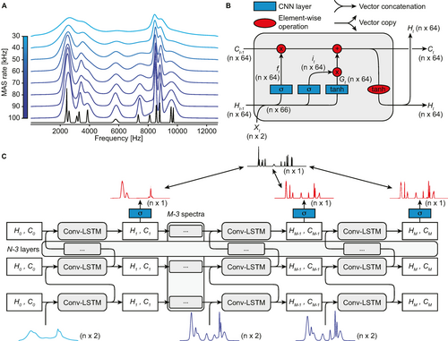
Data generation and signal processing. (A) Example of generated isotropic (black) and variable-rate MAS (blue) spectra. Here the top and bottom-most MAS spectra correspond to MAS rates of 30 and 100 kHz, respectively. (B) Convolutional LSTM cell used to process a spectrum, according to the overall scheme shown in (C) which describes the complete processing of the M=8 MAS spectra each containing n points in (A) with N LSTM layers to obtain predicted isotropic spectra. The initial cell state vectors H0 and C0 are described in the text. MAS spectra are encoded as vectors with two channels, the first one being the real part of the spectrum and the second one containing the MAS rate at each point. After the last layer, the hidden state Ht is processed with a CNN with sigmoidal activation function (blue square) to produce the prediction at each step (red spectra). When training, the predictions at each step are compared with the target isotropic spectrum (black spectrum), as indicated by the double arrow lines.
The architecture of the LSTM cell used here is described in Figure 1B (and is described in detail in the Experimental). The two main differences compared to the original description of LSTM14a are the use of CNN layers to process the inputs and the removal of the output gate. The former allows the processing of spectral data without the need for fixed input size and independently of the particular frequencies of peaks observed, while presence of the latter was found to be unnecessary since the isotropic spectrum is directly encoded into the memory of the LSTM network Ct and Ht, and does not require decoding that depends on the last MAS spectrum fed to the network (see Figure S3).
Figure 1C shows the complete processing pipeline performed by PIPNet in order to obtain the predicted isotropic spectrum from the set of MAS spectra shown in Figure 1A. At each step, another MAS spectrum from the set with a different rate is used as input to the network to update the state vectors of the LSTM cells. The spectra are fed into the process in order of increasing MAS rate, until all the spectra in the set (8 in Figure 1A, but 24 in the actual model training process) have been input. After each step, the state vector  of the final layer is processed by a final CNN layer to yield the predicted isotropic spectrum.
In order to obtain the uncertainty of the predicted isotropic spectra, PIPNet is a committee model made up of 16 neural networks with identical architectures, but each trained on completely independent synthetic data. At inference, the mean over the 16 predictions yields the predicted isotropic spectrum, and the standard deviation gives an indication of the uncertainty associated to the prediction at each point in the spectrum. Notably, uncertainty on the order of the predicted intensity highlights regions where the predicted spectrum is unreliable.
Figure 2A shows the evolution of the loss function, corresponding to the mean absolute error (MAE) between the predicted and ground-truth isotropic spectra, during the model training. The significant changes of scale in the loss after 320 000 and 800 000 training samples per model reflect the changes in the weighting of the loss function (see methods section). This was performed in order to promote the detection of peaks at the beginning of the training by decreasing the importance of the prediction in empty regions of the isotropic spectra. Figure 2B shows the comparison of the predictions obtained after training each model on 16 000, 800 000, 1 600 000, 2 400 000, 3 200 000 and 4 000 000 sets of MAS spectra. Significant improvement of the predictions can be seen until 1 600 000 training samples, after which the model was considered to have converged. This is reflected both by the plateau in the loss function in Figure 2A and by the obtained predictions for the example shown in Figure 2B, where the five peaks between 3500 and 5000 Hz were found to be captured by the model only after 1 600 000 training samples (although with different intensities). After that point, the isotropic spectra obtained did not display any significant change with increased amounts of training data. Nonetheless, we selected the final model at the end of the full training process, i.e., after 4 000 000 training samples per model.
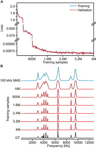
Model training. (A) Evolution of the loss function during model training. The large changes after 320 000 and 800 000 training samples per model correspond to the changes in loss function applied as described in the methods section. (B) Synthetic 100 kHz MAS spectrum (blue) and its associated ground-truth (GT) isotropic spectrum (black) compared to predictions of the model trained on 16 000, 800 000, 1 600 000, 2 400 000, 3 200 000 and 4 000 000 samples (red). The shaded areas in the predicted spectra indicate the standard deviation between the 16 neural networks making up the committee model.
Figure 3 displays the behavior of the model with different numbers of isotropic peaks, MAS dependences and levels of noise. The model was found to be robust to the number of peaks, with each peak resulting in a similar increase of the MAE between predicted and ground-truth isotropic spectra (see Figure 3A). As seen in Figure 3D, the number of peaks is generally correctly captured both for sparse and more crowded spectra. In instances where different peaks are not captured, they are typically found to coalesce into a single, broader peak.
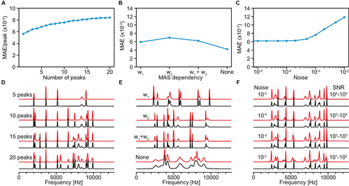
Model evaluation. (A–C) MAE between predictions and ground-truth isotropic spectra for 1 024 samples and (D–F), illustrative comparisons of predicted (red) and ground-truth (black) isotropic spectra with various (A), (D) number of peaks, (B), (E) MAS dependences (w1: first-order, w2: second-order), and (C), (F) noise levels. The MAE in (A) is normalized by the number of peaks. The typical range of signal-to-noise ratio (SNR) in 100 kHz MAS spectra corresponding to each level of noise is indicated in (F).
Figures 3B and 3E highlight the ability of the model to capture both first- and second-order MAS dependence of linewidths and shifts in MAS spectra, as well as combined first- and second-order dependence. A purely second-order MAS dependence was found to slightly raise the error between inferred and ground-truth isotropic spectra. In addition, using a set of identical spectra with different MAS rates (no MAS dependence) was found to result in only very marginal amounts of unexpected sharpening of peaks arising from overfitting of the model, seen in the region around 8000 Hz in Figure 3E. This indicates that PIPNet is robust to different MAS dependences.
Figures 3C and 3F show the robustness with respect to the level of noise in the MAS spectra. The MAE between inferred and ground-truth isotropic spectra was found to increase with noise levels of 10−3 and above, corresponding to a signal-to-noise ratio (SNR) of 1 000 and below in 100 kHz MAS spectra. We find that the predicted spectra visually display no significant perturbations down to a SNR of 100, below which some noise and uncertainties start to appear in the inferred spectra. Importantly, the model is still able to correctly identify the regions containing signals from pure noise down to a SNR of 10. Experimental fast MAS spectra of pure organic solids typically have SNR ≈1000. Artifacts are thus expected to appear only with low signal-to-noise ratio spectra, and would typically be associated with a high uncertainty (see Figure 3F). We found that the false positive rate in predicted spectra was under 1 % up to a noise level of 10−3 (SNR down to 100), and was found to be 22 % with a noise level of 10−2 (SNR of 10) (see Figure S4).
The model was also found to be robust to perturbations in the MAS-dependent linewidth, shift, number of MAS spectra and range of MAS rates selected (see Figure S4 and S5).
Figure 4 shows the isotropic spectra obtained from eight experimental sets of variable rate MAS spectra recorded on different compounds (detailed in the Experimental) in comparison to the corresponding 100 kHz MAS spectra. We note that the spectra obtained using PIPNet from these two-dimensional datasets were found to be similar to the parametrically fitted isotropic spectra, while notably displaying fewer artifacts (see Figure S6).
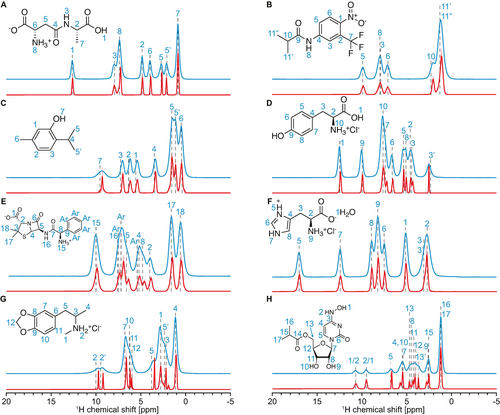
Predictions on experimental data. Experimental 100 kHz MAS spectra (blue) and isotropic spectra (red) of (A) β-AspAla, (B) flutamide, (C) thymol, (D) L-tyrosine hydrochloride, (E) ampicillin, (F) L-histidine hydrochloride monohydrate, (G) MDMA hydrochloride and (H) molnupiravir. The isotropic spectra were obtained for each compound from a set of between 31 and 41 MAS spectra recorded at rates between 20 and 100 kHz (as detailed in the methods section) using the model presented here. The assignment of the 100 kHz spectra, based on two-dimensional experiments (see Experimental), is indicated with vertical dashed black lines and blue numbers. In (H), the assignment of protons 1 and 2 is ambiguous.
The samples are microcrystalline forms of β-AspAla, flutamide, thymol, L-tyrosine hydrochloride, ampicillin, L-histidine hydrochloride monohydrate, MDMA hydrochloride and molnupiravir. The assignment and MAS datasets of β-AspAla, flutamide, thymol, L-tyrosine hydrochloride and ampicillin have already been reported previously.9, 16 The 1H and 13C assignment of MDMA hydrochloride and molnupiravir are done here as described in the Experimental, based on the acquisition of 100 kHz 0.7 mm 1D 13C CPMAS and 1H MAS spectra, 2D 1H-13C hCH17 and 1H-13C INADEQUATE spectra,18 DFT chemical shift calculations for MDMA and the probabilistic assignment approach of Cordova et al.19 (see Figure S1). A DNP enhanced INADEQUATE spectrum18 was recoded for MDMA (Figure S1) at 9.4 T in a 3.2 mm DNP probe at 100 K.
If we look at the case of L-tyrosine hydrochloride (Figure 4D) as a representative example, the expected number of peaks is retrieved and the peak positions match expectations from assignments carried out using 2D methods (see Experimental). The observed linewidths in the isotropic spectrum are very significantly narrower than the 100 kHz MAS spectrum, with full widths at half maximum (FWHM) between 62 and 250 Hz (0.08 and 0.32 ppm).
We note that while the obtained isotropic spectra generally display sharper lineshapes than those measured at the highest MAS rates, finite linewidths are still anticipated, as we expect distributions of the isotropic shifts due to the presence of more or less structural disorder in the sample. Isotropic shift distributions will also be caused by anisotropic bulk magnetic susceptibility (ABMS) effects,10 or as a result of imperfect B0 homogeneity. Importantly, no significant artifacts are seen in the isotropic spectra obtained. This behavior is seen in general across all eight samples in Figure 4. The linewidths observed in the isotopic spectrum are in line with expectations from a previous analysis of the MAS dependence of the measured linewidths of the resolved peaks (1 and 3′) given in Figure 14 of ref. 3b. It is especially notable that the isotropic spectrum predicted from the variable MAS dataset correctly identifies the 7 peaks present in the crowded spectral between 3 and 9 ppm, that are not resolved in the 100 kHz MAS spectrum.
It is important to note that PIPNet is not just identifying potential peaks and replacing them with uniformly narrow lines. We notably see in the cases of flutamide (Figure 4B) that there is only minor narrowing in the isotropic spectrum as compared to the 100 kHz MAS spectrum (see Table S5 for a list of resolved linewidths measured in both the 100 kHz MAS spectra and the isotropic spectra, for all eight compounds). Similar behavior was also observed using the parametric fitting approach (Figure S6), and we thus conclude that these peaks are dominated by chemical shift broadening and not MAS dependent dipolar broadening. We note that for ampicillin we also see only limited narrowing in the isotropic spectrum from PIPNet. In this case this in contrast with the parametric fitting approach, which produced narrower lines (Figure S6, Table S5). Here we suspect that the parametric fitting approach might be overfitting, and this is a good example of the more general and robust nature of the PIPNet model.
In addition to the six compounds previously reported,9 here we have obtained isotropic spectra for two additional molecular solids, MDMA hydrochloride and molnupiravir (Figure 4F and 4G, respectively). For MDMA hydrochloride, the expected peaks were clearly identified, except potentially for one in the aromatic (protons 7–12) regions of the spectrum. However, as seen in the HETCOR spectrum of the compound (Figure S1 and dashed vertical lines in Figure 4G), protons 10 and 11 display very similar chemical shifts, suggesting that the peaks might overlap in the isotropic spectrum. The isotropic spectrum of molnupiravir displayed all expected peaks. In particular, the two peaks in the region between 2 and 3 ppm are clearly identified from the PIPNet spectrum, while the fitted isotropic spectrum predicts only one broader peak (Figure S6). This highlights one limitation of the fitted model, as the presence of two isotropic peaks can be seen from the increasing asymmetry of the corresponding peak in the set of MAS spectra with increasing rate (Figure S2H), which corresponds to the two underlying isotropic peaks having different MAS-dependent shifts and/or broadenings. Considering multiple different MAS-dependent shifts in a single spectral region is thus critical here in order to correctly describe the experimental spectra as a function of MAS rate. While this is not captured by the fitted model due to the assumption that only one MAS-dependent shift is assigned to each fitted region, PIPNet makes no such assumption and thus is able to identify the two distinct resonances.
In summary, the isotropic spectra inferred by PIPNet from the experimental variable rate MAS datasets were found to display the expected number of peaks, without any prior information given about the sample measured. No significant artifacts were identified in the inferred spectra, highlighting the increased generality and robustness of the deep learning model compared to the previous fitted approach.
Figure 5 shows the comparison between the chemical shifts of 32 selected peaks from the compounds studied here, and Figure S7 compares the linewidths obtained, using the deep learning approach presented here with the positions observed at 100 kHz MAS, and with the fitted approach. We find strong correlations between the observed peak positions with the three methods, with a root-mean-square error of 0.060 ppm (≈50 Hz) and a R2 coefficient above 0.999. We note that this is not a direct metric of the accuracy of our model, as the 100 kHz MAS peak positions are not at exactly the isotropic shifts,3b, 3c, 6a, 8a, 8b and the fitting approach also suffers from shortcomings as mentioned above. The consistency between the three results does however strongly suggest that the method allows measurement of resolved isotropic shifts to within an error of 0.060 ppm. In Figure 5B, differences appear at discrete values in steps of ≈0.03 ppm, corresponding to the spectral resolution. If needed, more accurate peak maxima could be obtained by increasing the spectral resolution through zero-padding before running the prediction, or by applying more advanced peak picking approaches to the isotropic spectrum,13f Figure S7 and Table S5 suggests that linewidths are generally predicted to be broader using PIPNet than with the fitting approach. Because the model was found able to predict linewidths as low as 57 Hz (0.07 ppm) (see Table S6), we expect these differences to arise from approximations present in the fitted approach leading to a degree of overfitting, and not from incomplete removal of MAS-dependent broadening by the machine learning model.
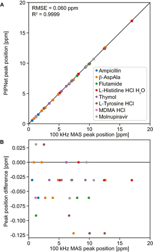
Predicted peak positions. (A) Comparison of the position of selected isolated peaks in the 100 kHz MAS and those in the isotropic spectra. (B) Difference in position of the peaks shown in (A). The black lines indicate perfect correlation.
As seen in Figure S8, the relative integrals of different spectral regions are retained in the predicted isotropic spectra compared to the experimental 100 kHz MAS spectra, with a deviation of less than ≈5 % of the total integral for all compounds.
An additional useful feature of the model presented here is the ability to predict spectra with linewidths comparable to high MAS rates (above 100 kHz) using only the lower MAS rate experimental spectra recorded. As shown in Figure 6, using only experimental spectra measured between 30 and 40–50 kHz, the model was found to generate a spectrum that is sharper than the experimental 100 kHz MAS spectra of L-tyrosine hydrochloride and β-AspAla. Similar examples for the other 6 compounds are shown in Figure S9. This highlights an alternative use of the model to obtain resolved spectra without the hardware needed to perform experiments at the highest MAS rates. In particular, this opens up the possibility to combine higher sensitivity of NMR experiments performed on samples prepared in, e.g., 1.3 mm or 1.9 mm diameter rotors with resolution corresponding to 100 kHz MAS, which is only currently attainable using smaller 0.7 mm diameter rotors. An example for L-histidine hydrochloride monohydrate obtained on a 1.3 mm MAS probe with 16 rates from 30 to 60 kHz is shown in Figure S10. Figure 6 shows that adding faster MAS spectra consistently leads to increased resolution of the predicted isotropic spectra until 80 kHz, after which the predictions were generally found to converge here. (It will be interesting to see what happens at even higher experimental MAS rates in the future).
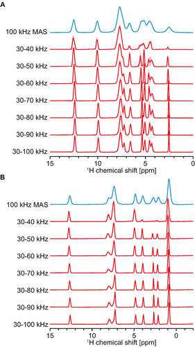
Isotropic spectra from different ranges of experimental MAS rates collected in 2 kHz increments. 100 kHz MAS spectra (blue) and isotropic spectra (red) obtained from different ranges of MAS rates for (A) L-tyrosine hydrochloride and (B) β-AspAla. The range of MAS rates used is indicated next to each isotropic spectrum.
Figure S11 suggests that using a lower number of experimental spectra while retaining the range of MAS rates used (40 to 100 kHz in Figure S11) leads to only marginal changes in the isotropic spectra obtained, up to increments of 10 kHz between measured MAS spectra. In light of this result and those shown in Figure 6 and Figure S9, we consider that converged isotropic spectra can typically be obtained using spectra from 30 to at least 80 kHz MAS rate, in increments of up to 10 kHz. We note that, in general, a minimum of 5 spectra are typically required to obtain meaningful isotropic spectra (see Figure S3). The quality of the isotropic spectra obtained is nonetheless expected to be higher using a larger range of MAS rates and a higher number of MAS spectra.
Conclusion
Here we have developed PIPNet, a deep learning approach to predict isotropic 1H NMR spectra of solids from a two-dimensional dataset of variable rate MAS spectra, using a convolutional recurrent deep neural network with modified convolutional LSTM layers. The model is able to reliably predict linewidths on par with a previously introduced fitting approach, while bypassing several limitations of the latter approach and at a fraction of the computational cost, leading to faster and improved predictions.
The model was applied to sets of MAS spectra for eight molecular solids and showed marked resolution improvements compared to the highest MAS rates available, with linewidths down to 57 Hz. In addition, even using only relatively low MAS rates (30–50 kHz) as input for the model led to predictions with linewidths comparable to fast MAS (>100 kHz), which opens up the possibility to obtain well-resolved 1H spectra for molecular solids from experimental data recorded at spinning rates accessible on less specialized hardware, such as, e.g., 1.3 mm MAS probes.
The spectra obtained using the PIPNet model from complete sets of variable rate MAS data up to 100 kHz MAS yield the best resolved 1H spectra of molecular solids recorded to date, and we anticipate that access to even faster spinning rates in the future will further improve the robustness of this method. The model is freely available at https://github.com/manucordova/PIPNet.
Acknowledgments
This work was supported by Swiss National Science Foundation grants 200020_212046, and NCCR MARVEL.
Conflict of interest
The authors declare no conflict of interest.
Open Research
Data Availability Statement
The data that support the findings of this study are openly available in the Materialscloud repository at https://doi.org/10.24435/materialscloud:a7-59.


