Contrasting Historical and Physical Perspectives in Asymmetric Catalysis: ΔΔG≠ versus Enantiomeric Excess
Abstract
With the rise of machine learning (ML), the modeling of chemical systems has reached a new era and has the potential to revolutionize how we understand and predict chemical reactions. Here, we probe the historic dependence on utilizing enantiomeric excess (ee) as a target variable and discuss the benefits of using relative Gibbs free activation energies (ΔΔG≠), grounded firmly in transition-state theory, emphasizing practical benefits for chemists. This perspective is intended to discuss best practices that enhance modeling efforts especially for chemists with an experimental background in asymmetric catalysis that wish to explore modelling of their data. We outline the enhanced modeling performance using ΔΔG≠, escaping physical limitations, addressing temperature effects, managing non-linear error propagation, adjusting for data distributions and how to deal with unphysical predictions,in order to streamline modeling for the practical chemist and provide simple guidelines to strong statistical tools. For this endeavor, we gathered ten datasets from the literature covering very different reaction types. We evaluated the datasets using fingerprint-, descriptor-, and graph neural network-based models. Our results highlight the distinction in performance among varying model complexities with respect to the target representation, emphasizing practical benefits for chemists.
1 Introduction
Enantioselective catalysis is a challenging yet essential aspect of synthesis, for example, of pharmaceutically active compounds, and represents a critical hurdle towards developing and marketing these products. The precision required in the process makes the quest for highly selective catalysts a formidable task. However, methods such as computational modeling offer promising avenues to streamline the process and expedite discovery and optimization cycles. Computational modeling, a sophisticated tool for unraveling complex catalytic mechanisms, acts as an innovative conduit for better understanding these phenomena, subsequently aiding the development of improved catalysts.
Although the incorporation of machine learning (ML) in catalyst discovery and optimization is a comparatively newer modeling trend, it should be noted that most of the underlying principles have been established over the last several decades. Both ligand-based and quantitative structure–activity relationship models have been used for over thirty years, often under the umbrella terms of chemometrics or cheminformatics, setting a solid foundation for the integration of AI in chemistry.1 The “newness” or revival of ML can be attributed to the significant rise in processing power of devices like graphics processing units, access to more extensive and information-rich data sets and new approaches to molecular representation.2 Together, these developments enhance the accuracy and predictive power made possible by ML.
However, as the merger of ML and enantioselective catalysis is still in its relative infancy, best practices for its successful application are yet to be firmly established. While preliminary guidelines exist for implementing ML in chemistry and other fields, careful validation and methodical clarity will be needed to ensure its reliable application in catalyst discovery and optimization. Scientists are actively contributing to this field, setting out to establish these best practices and expand the potential of this exciting interdisciplinary approach.3-5 When modeling enantioselective reactions, it is crucial to consider how the target variable is represented, with options including ee, enantiomeric ratio (er), and ΔΔG≠. Each of these can be derived from one another and represent different aspects of the same underlying data, as long as the tenets of transition state theory are valid. In this discussion, we advocate for the use of ΔΔG≠ when aiming for models that not only provide chemically meaningful insights but are also robust and generalizable across a variety of conditions. It is important to emphasize that linear regression and other modeling techniques allow for a wide array of transformations on both the target variables and the predictors. This flexibility enables the exploration of various transformations, such as logarithmic, polynomial, sigmoid, and Box-Cox,6 depending on the specific analytical needs and data characteristics.
Both, ee and er, are experimental quantities used to describe the selectivity and efficiency of asymmetric catalysts in producing one enantiomer over the other in an enantioselective reaction. However, they have different origins, historical uses, and reasons for their application as ee has historically been used in asymmetric catalysis and has its roots in the early days of enantiomer separation and analysis.7 It is the difference between the mole fractions of the two enantiomers in the product mixture. The ee is typically expressed as a percentage ranging from 0 % (racemic mixture) to 100 % (single enantiomer). Enantiomeric excess was historically introduced as a simple and intuitive way to describe enantioselectivity because it is a quantity that is proportional to the optical purity, e.g., rotation of linear-polarized light of a sample relative to that of the pure enantiomer. Conversely, the er is defined as the ratio of the percentages of each enantiomer in a mixture,8 which is proportional to the rate constants for forming each enantiomer. Thus, using er emerged as an alternative to ee due to its direct measurability in high-performance liquid chromatography, particularly in kinetic resolutions and asymmetric catalysis, where the two enantiomers′ formation rate is more relevant.9
In many cases, catalyzed enantioselective reactions are characterized by an irreversible (i.e., stereo-defining) progression through a transition structure (derived from the concepts of transition-state theory, TST) and the product ratio only depends on the difference of the diastereomeric transition structure free energies. Thus, ΔΔG≠ as the relative free activation energy difference of the enantio-determining pathways translates into the product‘s chiral purity. In contrast, experimental observables of chiral purity such as ee and er are indirect representations of the underlying cause that determines chiral purity, i.e., ΔΔG≠. For regression modeling, targeting a quantity that directly measures the underlying cause of a process, such as ΔΔG≠, may yield models that are more physically meaningful and insightful. In reality, other factors can influence the chiral purity of reaction products, such as side reactions that lead to product racemization or the formation of enantiomeric products by different mechanisms (such as a competition between enantiospecific reactions of enantiomerically enriched starting materials). An example of a catalyzed reaction that converts an achiral starting material to a chiral product is the Corey-Bakshi-Shibata (CBS) reduction (Scheme 1).10
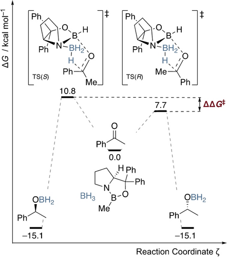
Exemplary potential free energy surface showing the enantioselective reduction of acetophenone to the corresponding chiral benzyl alcohol via CBS reduction. The selectivity is determined by the difference in free energy of the diastereomeric transition structures (TSS and TSR) ΔΔG≠.11 Relative free energies at the B3LYP−D3(BJ)/6–311+G(d,p)-SMD(THF)//B3LYP−D3(BJ)/6–311G(d,p) level of theory.12-16
In the CBS reduction, a prochiral ketone is reduced with a chiral oxazaborolidine catalyst to yield a chiral alcohol. This reaction occurs through two diastereomeric transition structures. The difference in their free energy, represented as ΔΔG≠, dictates the chiral purity of the resulting product, i.e., the enantioselectivity of the reaction. In the example shown in Scheme 1, the reduction of acetophenone, the computed ΔΔG≠ is 3.1 kcal mol−1, which converts to an ee of 98.9 % at 25 °C. This is in reasonable agreement with the experimentally observed value of 97 % ee. Thus, the picture of competing transition structures serves as a useful bridge between the experimental observables ee or er and mechanistic concepts that are expressed in relative free energies.
Utilizing ΔΔG≠ values rather than ee values in molecular modeling can further be rationalized based on Linear Free Energy Relationships (LFERs)17-21 and the Bell−Evans−Polanyi principle,22, 23 as these concepts provide an understanding of the thermodynamic and kinetic factors influencing enantioselective reactions. The Bell−Evans−Polanyi principle asserts that the difference in activation energies between two reactions may be proportional to the difference in their reaction enthalpies.24 In the context of enantioselective processes, this principle implies that the difference in activation energies between the formation of two enantiomers (represented by ΔΔG≠) is related to the difference in their reaction energies (to the catalyst-bound product as the individual enantiomers have identical free energies). By incorporating ΔΔG≠ values into molecular modeling, a reasonably complete representation of thermodynamic and kinetic aspects can be achieved. Additionally, LFERs posit that the free reaction energy may correlate linearly with specific attributes of the reactants, be they steric or electronic. Historically, these steric and electronic factors were treated as separate entities in chemical interactions. However, contemporary understanding has advanced to integrate these two factors, leading to the emergence of the stereo-electronic effects concept.25 This convergence represents a significant advance in our current understanding and analysis of chemical reactions. It also is physically more sound as all such effects originate solely from electron distributions.
This concludes our outline of the relationship between ee and ΔΔG≠ with a proposal to use ΔΔG≠ as the target variable for modeling, as it is advantageous for several reasons:
-
Physicality: ΔΔG≠ possesses direct physical significance as it is the resulting quantity behind observed selectivities (see above), making it a pertinent choice for understanding the underlying processes and mechanisms (which would ideally be accompanied by transition state computations), while ee is more of a historic quantity.
-
Temperature: ΔΔG≠ incorporates temperature as a variable, which has proven to be an essential factor affecting selectivity in most catalyzed enantioselective reactions.26, 27 Only by using ΔΔG≠, the model can routinely capture temperature effects on the selectivity according to the underlying physical effects. We hypothesize that this results in more accurate predictions and comparabilities of stereoselectivities. Conversely, ee does not include its inherent temperature dependence, which may lead to less accurate models, because the temperature has to be provided as an extra input feature and additional context has to be learned by the model.
-
Limits: A key consideration when selecting between ee and ΔΔG≠ as target variables is their respective value ranges. While ee is by definition constrained to the limits −100 to +100 (for denoting the excess of R and S enantiomers), this restriction does not apply to ΔΔG≠ as shown in Figure 1
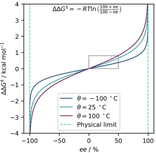 Figure 1
Illustration of the non-linear relationship between ee and the change in ΔΔG≠ at three temperatures. The green dashed lines represent the fundamental limits for ee, indicating that employing a model based on ee may yield implausible predictions if they occur over 100 %. In contrast, such restrictions are absent when utilizing ΔΔG≠ as the modeling target. The marked part of the Figure emphasizes the approximately linear region at low selectivities (<50 % ee). This highlights that the non-linearity between ee and ΔΔG≠ is especially noticeable at higher selectivities, which are more desirable.
. Although a model can in principle cover the entire range for both variables, predictions for ee from numerical models might extend beyond its meaningful range (if not explicitly constrained). Consequently, these predictions would have no real-world significance, as values below −100 or above +100 are not physically possible. In contrast, the absence of such limitations for ΔΔG≠ allows the model to make predictions across a much wider range of values, enhancing generalizability and ensuring that predictions maintain relevance in real-world scenarios.
-
Distribution: As a consequence of the non-linear relationship between ee and ΔΔG≠, the distribution of a data set changes, meaning that the way data points are spread or clustered can vary when converting between these domains (as illustrated in Figure 2
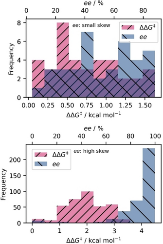 Figure 2
Histograms showing DS3 (small skew, top) and DS7 (high skew, bottom) in the ee (blue) and ΔΔG≠ (pink) domain. The purple region indicates where both (pink and blue) distributions overlap. Note that the a smaller skew is observed when looking at narrower selectivity ranges (top), compared to a wide-ranging dataset (bottom), where the skew gets larger to the non-linear transformation.
), typically resulting in more normally distributed data when expressed as ΔΔG≠. Unbalanced data sets can lead to clustering effects and misleading patterns. For instance, the common goodness of fit metric R2 (coefficient of determination) might be artificially high in strongly clustered data. A classic example of how fit metrics can be misleading for different data distributions is Anscombe's quartet.28 Furthermore, metrics such as R2 and RMSE are used to evaluate the quality of a model fit and the ability of a model to make predictions on unseen data, which we scaled by the all-mean prediction (the “null-model”). Both scores are affected by the transformation between ee and ΔΔG≠ (see below). In practical terms, minor errors in the 95–99 % ee range are critical, while large errors in the 1–50 % ee range are less relevant when evaluating enantioselectivity. Data clustering can also result in non-representative training-testing splits in small data sets, as often encountered in enantioselective catalysis, unfavorably affecting the generality of test set metrics. Notably, the non-linearity of the ee-to-ΔΔG≠ transformation only becomes pronounced at higher selectivities (Figure 1, bottom), i.e., for data<50 % ee the transformation makes little difference to the distribution.
In the following sections, we demonstrate the effect of each of these arguments using real-world data from the literature as well as from artificial data sets. While target transformations can have an important effect on model performance, we stress that different choices may be right depending on the context.29-32 For example, one upside of using ee is that it is intuitive to experimentalists, facilitating communication of model outcomes. However, this can also be achieved by modeling on ΔΔG≠ and then transforming predictions and metrics to the ee domain for more intuitive representation.33
In addressing the nuances of chemical data analysis, particularly the decision to use ee vs. ΔΔG≠ for modeling enantioselectivity, it is important to highlight the practical reasons for choosing ΔΔG≠. For chemists without extensive statistical training, ΔΔG≠ offers a straightforward and interpretable alternative. Unlike other transformations (e.g., log, Box-Cox),6 which require additional steps and expertise, ΔΔG≠ directly correlates with the underlying physical processes, making it more intuitive and easier to apply. These transformations are pivotal in linear regression models, where they serve to homogenize variance, thereby enhancing the reliability of statistical inferences. Such practices are not unique to chemistry but are extensively applied in various domains of data analysis. For instance, Box and Cox′s transformation is a well-known method for stabilizing variance in data that follow a non-normal distribution.6 Similarly, in bioinformatics, variance stabilization is crucial for analyzing microarray data, a topic explored by Huber and co-workers.34 By integrating these foundational concepts, our discussion on ee vs. ΔΔG≠ not only aligns with chemical specificity but also resonates with established statistical methods, thereby enriching our contextual framework within statistical modeling practices.
2 Benchmarking Methods
We collected data from the literature to investigate various aspects of the target transformation on real-world results in enantioselective catalysis that have been used for data-driven modeling. Our focus is on publications that utilize molecular descriptor-based models to compare the influence of featurization. Furthermore, we aimed for a representative selection with different data structures (i.e., combinatorial screening or traditional linear optimization) across a range of data set sizes commonly encountered in modeling enantioselectivity (about 20–1000 data points) and featuring examples from various types of catalytic reactions (Table 1).
Dataset |
Research groups |
Reaction |
Samples |
Available features |
|---|---|---|---|---|
DS147 |
Sigman, Biscoe |
Pd-phosphine catalyzed Alkyl-Suzuki coupling |
24 |
Descriptors |
DS248 |
Doyle |
Ni-BiOx/BiIm, photo-catalyzed Cross-electrophile coupling |
29 |
Descriptors |
DS349 |
Sigman, Toste |
DAP-catalyzed allenoate-Claisen rearrangement |
37 |
Descriptors |
DS450 |
Tsuji, Sidorov, Varnek, List |
IDPi-catalyzed Hydroalkoxylation |
80 |
SMILES, Descriptors |
DS551 |
Ackermann, Hong |
Pd+TDG, electrocatalyzed oxidative Heck reaction |
127 |
SMILES, Descriptors |
DS652 |
Toste, Sigman |
Triazole-PA-catalyzed cross-dehydrogenative coupling |
159 |
SMILES, Descriptors |
DS753 |
Sunoj |
Asymmetric hydrogenation |
371 |
SMILES, Descriptors |
DS854 |
Sunoj |
Pd-PyrOx-catalyzed relay-Heck reaction |
398 |
Descriptors |
DS955 |
Belyk, Sherer |
Phase transfer-catalyzed aza-Michael addition |
471 |
SMILES, Descriptors |
DS1056 |
Denmark |
CPA-catalyzed nucleophilic thiol addition |
1075 |
SMILES |
We employed three general classes of ML approaches to investigate the impact of target transformation on model performance:
1) For descriptor-based models, molecular features were utilized unchanged where available in the original publications. In data sets DS1–DS9, various steric and electronic descriptors were available from DFT computations. In DS9 and DS4-THF, 2D topological descriptors were used.
2) Morgan fingerprints with a radius of 2—meaning they capture the chemical environment up to two bonds away for each atom—were generated using the RDKit from the SMILES representations and folded to 1024 dimensions for fingerprint-based models.35 In data sets with several variable molecules (e.g., substrates and catalysts) present, the resulting fingerprints were added. Models for representations 1) and 2) were trained with various standard machine learning regressors as implemented in Scikit-learn36 on 50 different random 80 : 20 train:test splits of the data to obtain consistent model scores. Hyperparameter optimization was performed once for each model-feature set combination using repeated k-fold (four folds, five repetitions) cross-validation in the training set on the first 80 : 20 random split. The following linear regressors were used: Linear regression, ridge, Lasso, LassoLars, elastic net. The following non-linear regressors were used: random forest, gradient boosting, extra trees, kernel ridge, Gaussian processes, and k-nearest neighbors.37-46
3) Graph-based models were trained with molecular graphs that were generated from the provided SMILES representations, which were converted into molecular objects using the RDKit and subsequently constructed into molecular graphs with standard node and edge features (refer to Supporting Information for a comprehensive list). In instances with n SMILES, we generated a graph comprising n distinct, non-interconnected subgraphs embedded within the overall molecular graph. These graphs were then processed using a Graph Neural Network (GNN) to produce a molecular embedding after global pooling operation, which was fed into a feed-forward neural network (FFNN) (code is available free of charge, see below). For GNN and FFNN, we used Pytorch Geometric and Pytorch.57, 58 We conducted training for the model both with and without incorporating temperature as an extra input feature in the FFNN. This was done to account for the potential effects of temperature dependence, which was also of interest. We employed a Bayesian optimization approach via Optuna to optimize the hyperparameters of the GNN model.59 As an optimizer we used Adam with the Mean Squared Error (MSE) as a training metric. To avoid overfitting, we employed the early stopping technique. While cross-validation is a widely used method for model evaluation, it may not be the most suitable choice for small datasets and GNNs due to the constraints posed by limited data, high computational cost, and potential bias in the molecular structure encoded in the molecular graph. Instead, assessing the performance using multiple random states can provide a more reliable estimate of the model's generalization ability while overcoming these limitations. This approach involves randomly splitting the data into training and test sets multiple times (i.e., 500 times) and calculating the performance metrics for each split. The average performance across all random states provides a more robust estimate of the model's generalization capability while mitigating the challenges associated with cross-validation.
We divided the model performance evaluation into four categories: descriptor-based (separated into linear and non-linear models), fingerprint-based, and GNN. We computed the mean absolute error (MAE) on each dataset for each model and variation (including or not including temperature). To fairly scrutinize the disparity in performance between ΔΔG≠ and ee modeling, we transformed predictions from both into the er domain, which is mathematically possible without applying a capping threshold that could have led to potential distortions. To obtain comparable values across the data sets, we normalized the MAE between 0 and 1 by the MAE of an all-mean prediction.
3 Results
The transformation between ee and ΔΔG≠ is non-linear and thus affects the distribution of data sets. We investigated the effect of this transformation on the data structure using the skew score and the Kolmogorov–Smirnov (KS) test. The skew score quantifies the skewness, that is, the degree of asymmetry in a distribution with a positive value indicating a right-skewed distribution, i.e., leaning towards lower values. A skewness of 0 indicates that the data are perfectly symmetric, and deviations from 0 indicate asymmetry in either direction of the tested datasets. The Kolmogorov–Smirnov (KS) score indicates the difference between two distributions, with 0 indicating identical distributions and 1 indicating entirely different distributions. Here, we test the experimental selectivities against a normal distribution, i.e., lower scores indicate distributions closer to normal. It should be noted that data from traditional “linear” reaction optimization and reaction scope tables tend to be biased towards higher selectivities because experimentalists focus on more selective reactions when pursuing a new method. Screening methods such as combinatorial evaluation of all substrate/catalyst pairs tend to generate data with a relatively higher portion of less selective or lower-yielding results, which is favorable for ML modeling.60, 61 Accordingly, nearly all data sets display a negative skew (towards higher values) when expressed as ee. Averaged over all ten sources, the absolute skew score decreases from 1.2 to 0.35 by transforming from ee to ΔΔG≠, indicating a clear overall shift towards more symmetric data distributions in the free energy domain. Likewise, the KS decreases from 17 % to 11 % probability indicating that the data were not drawn from a normal distribution upon transformation of ee to ΔΔG≠. The differences are most pronounced in more extensive data sets (>100 samples) of traditional “linear” optimization and scope results (DS7, DS8). In smaller data sets (<100 samples), the differences are less pronounced but also less significant due to the low sample size. Denmark's CPA catalysis data set (DS10) is the biggest screening-type data set, containing the complete combinatorial evaluation of substrate/catalyst pairs. Interestingly, while the absolute skewness increases and switches from negative to positive by transformation to ΔΔG≠, the similarity to a normal distribution is still higher in the free energy domain (17 % vs. 8 %). Differences in data distribution are the smallest for data sets with lower overall selectivity (DS3) due to the approximate linearity between ee and ΔΔG≠ in that range (Figure 1, bottom). A summary of all distribution metrics is shown in Table 2.
Dataset |
ee |
ΔΔG≠ |
|skew (ΔΔG≠)| − |skew (ee)| |
N |
||
|---|---|---|---|---|---|---|
skew |
KS |
skew |
KS |
|||
DS1 |
−0.81 |
0.22 |
0.29 |
0.16 |
−0.52 |
24 |
DS2 |
0.03 |
0.19 |
0.31 |
0.22 |
0.28 |
29 |
DS3 |
−0.15 |
0.11 |
0.40 |
0.11 |
0.25 |
37 |
DS4 |
0.18 |
0.12 |
0.78 |
0.12 |
0.60 |
80 |
DS5 |
−1.49 |
0.29 |
−0.54 |
0.17 |
−0.95 |
127 |
DS6 |
−0.46 |
0.08 |
0.39 |
0.07 |
−0.07 |
159 |
DS7 |
−3.24 |
0.23 |
−0.04 |
0.05 |
−3.20 |
371 |
DS8 |
−3.54 |
0.22 |
−0.39 |
0.09 |
−3.15 |
398 |
DS9 |
−1.05 |
0.14 |
−0.60 |
0.09 |
−0.45 |
471 |
DS10 |
−0.54 |
0.17 |
0.86 |
0.08 |
0.32 |
1075 |
AVG |
−1.10 |
0.18 |
0.15 |
0.12 |
−0.69 |
277 |
A visual representation of the skew can be seen in Figure 2, in which a small skew (top, DS3) and a large skew (bottom, DS7) are shown between the ee and ΔΔG≠ domains. In the case of a small skew, the distributions look similar and evenly-distributed, while the large skew shows a normally-distributed dataset in ΔΔG≠ while being highly unbalanced in ee, as apparent from the large distribution density in the high ee range close to the maximum.
The detrimental effects of an unbalanced data set become clearly evident when examining a data set like DS7 (Figure 3). We simulate a model with an MAE of 5 % in the ee domain by adding random noise of that magnitude to the data (depicted in blue). Superficially, this score seems commendable, with a corresponding R2-score of 0.92. To the end-user, this might appear as a robust, “reliable” model. However, this is no longer the case when we transition to the more physically meaningful ΔΔG≠ domain where the “model's” inadequacies become evident: The scatter plot reveals a far less convincing fit, with an R2-score of only 0.49 (shown in magenta). In stark contrast, the opposite approach, constructing an artificial model with 5 % noise on the ΔΔG≠ values (R2-score of 0.98), translates seamlessly to the ee domain (R2-score of 0.99). This underscores the dangers of relying on seemingly “good” models without thoroughly probing their applicability across different domains. This is particularly relevant in the high ee regime where the largest errors occur, but which also is the most sought-after range for practical applications. We want to emphasize that any 5 % variance in % ee at the high end of the selectivity range would result in a significant impact in the ΔΔG≠ domain. This highlights the risk of trusting a model trained on ee with a relatively low MAE. Depending on where the model‘s main error lies, a large error in ΔΔG≠ at the high selectivity range cannot be prevented.
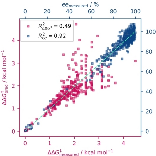
Scatter plot showing the data from DS7 as measured and “predicted” by adding random noise of ±5 % in ee (blue, top and right axis labels) and then calculating to the ΔΔG≠ domain (magenta, bottom and left axis labels). The light-green diagonal indicates optimal prediction.
Figure 4 underscores the significance of maintaining predictions within the physically meaningful domain ΔΔG≠ also from a practical perspective because the impact of an error in ee hinges on the specific selectivity range where the error transpires. An artificial data set is shown, and four specific “prediction” errors are highlighted (red bars): two with 0.2 kcal mol−1 ΔΔG≠ and two with 10 % ee, one each at a lower and a higher selectivity range. For constant ΔΔG≠ errors, this translates to either an error of 16.1 % ee at low selectivity (<40 % ee) or 0.6 % ee at high selectivity (>98 % ee), thus resembling acceptable uncertainties from an experimental point of view, that change accordingly depending on the selectivity. Conversely, the constant ee error may correspond to 0.2 or 1.3 kcal mol−1, i.e., a high error where higher precision would be needed and a low error where precision is less important.
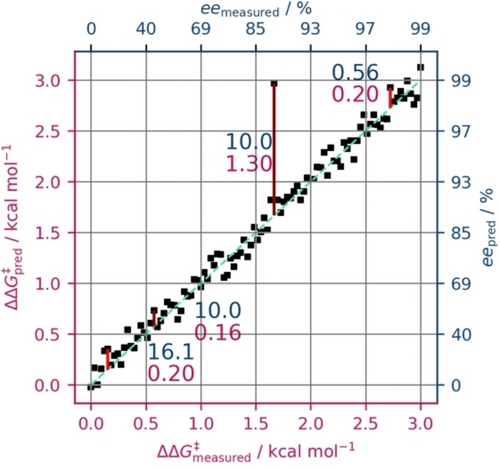
Scatter plot showing an artificial dataset (measured and predicted) in ΔΔG≠ along with its conversion to the ee domain (dark blue axis labels, scaled to the corresponding ΔΔG≠). The dashed light-green line indicates optimal prediction.
Concerning the value limits, model predictions exceeding 100 % ee account for about 4 % of all predictions performed for the models in this work. The frequency of such predictions largely depends on the number of entries with very high ee values in the training data. The conversion to ΔΔG≠ becomes arbitrarily large for values approaching 100 % and is undefined for ee values of 100 % and above. Thus, predictions in ee must be capped at a certain threshold before conversion (e.g., 99 % or 99.9 %) and selecting an appropriate capping threshold can significantly impact the model‘s metrics, potentially leading to misconceptions about its true performance. To investigate this effect, we looked at the model predictions for DS4 and varied the capping thresholds while calculating ΔΔG≠ derived from the predicted ee, and subsequently computed MAE in kcal mol−1. The results indicate an exponential growth in error with respect to the chosen threshold (Figure 5), illustrating the considerable influence of this seemingly innocuous parameter on the overall model evaluation. We suggest a capping threshold of 99.9 % when calculating ee back to ΔΔG≠, based on the elbow method.62 The chosen capping threshold can also be justified by typical experimental error ranges of enantiomeric ratios.
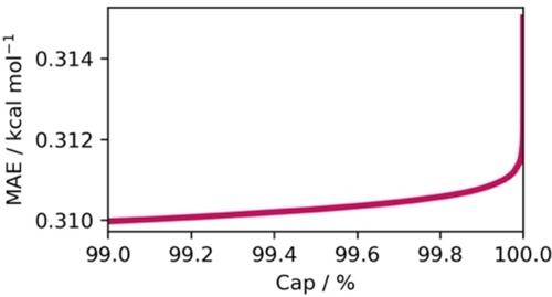
Error measured as MAE in kcal mol−1 with respect to the capping threshold (Cap) in % during the ΔΔG≠ conversion of predicted ee. The calculations were performed on DS4 with temperature included as a modeling feature in conjunction with our GNN model. Of all 175 k predictions, only 62 (0.35 %) were predicted over +100 % or below −100 % ee and subsequently capped.
We evaluate the impact of target transformation on general model performance by comparing the best of several standard ML regressors in four different categories, each modeled separately using either ee or ΔΔG≠ as targets for each of 11 data sets. The goal was not to achieve the best possible models or to compare models with the results from the respective original publications, but to have a consistent approach that allows a fair comparison among the data sets and target transformations. Thus, we do not discuss absolute model metrics such as MAE or R2, but rather relative MAEs after scaling all predictions by the mean baseline after transforming predictions to er (lower is better).
The performance evaluations shown in Figure 6 suggest that the discrepancy between modeling in the ee and ΔΔG≠ domain is generally small but not negligible. For nearly all sections (model type and dataset), modeling ΔΔG≠ appears to be superior to modeling ee; in the few cases where ee was superior to ΔΔG≠, the differences were only marginal. Generally, the differences between both domains were very prominent for some datasets, e.g., DS1, DS5, and DS10. This renders ΔΔG≠ the better choice of modeling domain compared to ee.
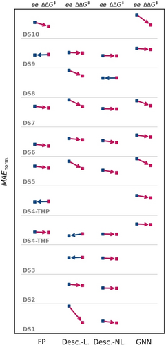
Performances for the best models for each dataset (stacked along the ordinate) in each method class (appended along the abscissa) with the respective modeling domain ee or ΔΔG≠. As a common performance metric between ee and ΔΔG≠, we chose the MAE in the er domain, normalized on the MAE of an all-mean-prediction to ensure values between 0 and 1. Performance points for each dataset and method are connected by an arrow, pointing to the lower-lying error, hence the better performing model; an arrow pointing towards the ee modeling (left) is colored in blue, while arrows pointing to modeling ΔΔG≠ (right) are colored red. Model classes are fingerprint-based (FP), descriptor-based (Desc.) with linear (L) or non-linear (NL) models, and graph neural network (GNN). In cases where no arrows are drawn, the combination of method and dataset was not available.
Notably, the improvement of modeling on ΔΔG≠ was more pronounced for linear, descriptor-based models (24 % improved relative MAE on average) than for non-linear or fingerprint-based models (6 and 10 % improved relative MAE, each), which is in line with an interpretation of linear descriptor-based models as an evolution of LFER, further suggesting that the transformation to ΔΔG≠ does lead to improved models. Note that perhaps similar improvements compared to ee could be achieved with other target transformations (see above), however, when working with small datasets optimizing the target transformation could lead of overfit models, as the target transformation has to be considered another hyperparameter of the model. Especially in real-world modeling, where practical chemists create or use the output of trained models, it would be wise to use a target transformation that is familiar to practical chemists and makes decision support via modeling easier to convey. Conversely, non-linear models may be able to learn the effect of the non-linear nature of ee given a physically-based molecular representation. Despite this, GNN models also showed an average relative MAE improvement of 20 % when using ΔΔG≠ as targets.
As Figure 7 indicates, incorporating temperature as an additional modeling feature is generally not of major importance, but the differences are often subtle when excluding temperature, which is not statistically relevant. However, for GNNs using temperature as an extra input feature seems superior in every case, and for DS5 a clear preference to include the temperature is observed. This is bolstered by our quantitative evaluation, which indicates that excluding temperature from modelling is favorable for FP-based models by 0.5 %. Descriptor-based models are not influenced by inclusion or exclusion of temperature as an additional modelling parameter, and have an average difference of 0 %. Inclusion of temperature for GNN-based models is beneficial in modelling attempts by 5.9 %.
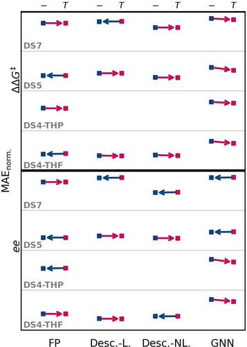
Performances for the best models for each data set (for modeling in ee and ΔΔG≠ stacked along the ordinate) in each method class (appended along the abscissa) with differentiation between exclusion (−) or inclusion (T) of temperature as an additional modeling feature. The MAE used for evaluation is normalized on the MAE of an all-mean prediction to ensure values between 0 and 1. Performance points for each dataset and method are connected by an arrow, pointing to the lower-lying error. Hence the better performing model is indicated; an arrow directed towards the without temperature modeling (left) is colored in blue, while arrows pointing to with temperature modeling (right) are red colorized. Model categories are the same as in Figure 6.
4 Conclusions
In organic chemistry, particularly in asymmetric organocatalysis, we face a reporting bias (publication bias), which refers to the selective publication and reporting of results that exhibit high yields, enantioselectivities, and reaction rates. This bias may arise from various factors, such as the desire to present new, impactful findings or the pressure to publish positive results to secure funding and advance careers. Consequently, what is perceived as less favorable or less exciting results may be less often reported in full or possibly not at all, leading to a skewed understanding of catalysts′ true scope and limitations in asymmetric reactions. This leads to an incomplete understanding: A biased representation of results in the literature can hinder the development of a comprehensive understanding of catalysts, mechanisms and their limitations, especially when using ML. This can lead to a distorted view and biased models. The lack of transparency and reporting negative or less favorable results can slow scientific progress, as such data are valuable to model training. In data modeling, this reporting bias leads to data markedly skewed to higher selectivities (or yields). This is unfortunate because an objective distribution would even be expected to lead to lower selectivities, as experience shows that achieving high selectivity is difficult and most “random” combinations of catalyst and substrate will result in no or low selectivity. However, for a model to truly learn the structure-selectivity relationships of a reaction, the reasons why specific catalysts result in low selectivity are equally as important as those leading to high selectivity.63 Especially when thinking about decision support the statistical tool at hand should provide guidelines for the practical chemist. As shown in Figure 2, the resulting unbalanced data sets can be compensated when staying in the ΔΔG≠ domain.
To truly identify a model of potential use, the domain has to be considered, as models resulting in a good fit in the ee domain do not necessarily remain useful when applying non-linear transformations like, to, e.g., the ΔΔG≠ domain. Since the error transformation between both domains is non-linear, comparing models from ee domain with those from utilizing non-linear transformations, i.e., ΔΔG≠, becomes challenging. It is thus advisable to directly model in the physically grounded ΔΔG≠ domain, which aligns with the overall superiority in modeling performance. Using one domain and not relying on transformations between domains, such as non-linear transformations like ΔΔG≠, also eliminates the need for a cutoff threshold, which we discuss in Figure 5. This simplification is particularly beneficial for chemists without extensive statistical training, making the modeling process more accessible and the results more interpretable. While the impact of including temperature as an additional input feature is subtle, we still advocate for its incorporation to enhance model accuracy.
The process of target transformations, as discussed in this work, is crucial not only in asymmetric catalysis but also in kinetics, specifically in reaction rates. Recently, Votsmeier et al. used the hyperbolic sine function to model chemical kinetics through transformation.64 A compelling extension of our research could involve examining the variations in model explanations such as attention maps, saliency maps, integrated gradients, and layer-wise relevance propagation methods, all contingent on the specific modeling domain further improving trust in the reasoning of statistical tools and hence increasing impact with increased usage in the laboratory. We hypothesize that a model trained with physically sound principles would yield more reliable and practically beneficial explanations, which could, for example, be leveraged for catalyst optimization and reduces the chance for an overfitted model, by rendering the target transformation optimization obsolete.
Disclaimer
The opinions expressed in this publication are the view of the author(s) and do not necessarily reflect the opinions or views of Angewandte Chemie International Edition/Angewandte Chemie, the Publisher, the GDCh, or the affiliated editors.
Acknowledgments
This work was supported by the Deutsche Forschungs-gemeinschaft within the priority program “Utilization and Development of Machine Learning for Molecular Applications—Molecular Machine Learning” (SPP 2363, Schr 597/41-1 and GE 3064/2-1). M.R. thanks the Fonds der Chemischen Industrie for doctoral scholarship. We thank Dennis Gerbig (JLU Giessen) for fruitful discussions. Open Access funding enabled and organized by Projekt DEAL.
Conflict of Interests
The authors declare no conflict of interest.
Open Research
Data Availability Statement
The authors have cited additional references within the Supporting Information.30, 31 A more detailed description of the datasets, modeling details, and selected plots for specific datasets are included. The data and code is available free of charge at https://github.com/prs-group/Contrasting-Historical-and-Physical-Perspectives-in-Asymmetric-Catalysis.git.


