Subjective life expectancies, time preference heterogeneity, and wealth inequality
Abstract
This paper examines how objective and subjective heterogeneity in life expectancy affects savings behavior of healthy and unhealthy people. Using data from the Health and Retirement Study, we first document systematic biases in survival beliefs across self-reported health: those in poor health not only have a shorter actual lifespan but also underestimate their remaining life time. To gauge the effect on savings behavior and wealth accumulation, we use an overlapping-generations model where survival probabilities and beliefs evolve according to a health and survival process estimated from data. We conclude that differences in life expectancy are important to understand savings behavior, and that the belief biases, especially among the unhealthy, can explain up to a fifth of the observed health-wealth gap.
1 Introduction
The determinants of the wealth distribution are of fundamental interest to economists. Standard consumption/savings theory predicts that people who place a larger weight on future states will be wealthier than people who are more impatient, all else equal. This paper explores one reason to put a higher weight on the future: the higher probability to survive to old age.
However, an individual's consumption/savings decision is not necessarily guided by the objective (statistical) survival probability but rather the individual's beliefs about survival. The first contribution of this paper is to document new facts about a within-cohort steepness bias in survival beliefs: people overestimate the health gradient of survival.
It has previously been shown (e.g., Hamermesh (1985), Elder (2013), Ludwig and Zimper (2013), Heimer, Myrseth, and Schoenle (2019)) that there is a systematic flatness bias over age: younger people tend to underestimate their survival probabilities, while older people overestimate their chances of a long life. We show that within a cohort, individuals in bad health not only have a shorter expected life span but are also relatively more downward biased about their survival chances, while individuals in good health, and thus with higher survival probability display an upward bias. These systematic biases exacerbate the life expectancy heterogeneity in the population.
The differences in beliefs about survival translate into time preference heterogeneity in the population. Our second contribution is to quantify this heterogeneity and its implications for savings and wealth accumulation in an overlapping-generations model. With a stochastic health and survival process, the effective discount rate varies depending on age, health, and the forecast horizon. Over a 1-year horizon, the effective discount rate for 50-year-olds ranges from 2% for an individual in best health to around 20% for an individual in worst health. At a 10-year horizon, this gap shrinks somewhat but still amounts to 8 percentage points between best and worst health. For 70-year-olds in worst versus best health state, the difference at the 10-year horizon is close to 10 percentage points. This resulting time preference heterogeneity is in line with the dispersion (Calvet, Campbell, Gomes, and Sodini (2021)) and the age gradient (Kureishi, Paule-Paludkiewicz, Tsujiyama, and Wakabayashi (2021)) of the time preference distribution found in other empirical studies.
To gauge the quantitative effect of survival heterogeneity on savings behavior and wealth accumulation, we use an overlapping-generations general-equilibrium model with uninsurable idiosyncratic shocks. Agents face heterogeneous survival risk that depends on their age and current health state, and are subject to health shocks that follow a process estimated from data. The current health state also affects labor earnings and medical expenditure risk. Besides this uncertainty, we additionally include standard persistent and transitory shocks to labor productivity during working age. After agents reach a fixed retirement age, they are entitled to retirement benefits mimicking the US social security system. Finally, our model includes probabilistic bequests that feature intergenerational persistence of income and wealth. We purposely use an otherwise standard model of consumption/savings to establish a benchmark and focus on the survival heterogeneity savings channel.
We compare three scenarios. The first scenario is a standard model in which there is no health risk: all agents face the same labor earnings risk, the same medical expenditure risk, and the same survival risk, and thus have the same effective discount factor, conditional on age. In the second scenario, we introduce health risk that affects labor earnings and medical expenditures. In terms of survival risk, individuals are perfectly informed about their true survival probability conditional on health and age. In the third scenario, agents believe and act according to their subjective survival beliefs. Thus, our analysis is designed to answer the question: what if we turned off the discount factor heterogeneity implied by the biases in survival beliefs we uncovered in the empirical part? Would savings patterns look quantitatively different?
The simulations show that the survival expectation channel is important for understanding wealth accumulation. Not surprisingly, agents in bad health, and thus with a shorter expected life span save less than their healthy counterparts, and the differences in savings rates are large. For example, for 60-year-olds in the middle of the wealth distribution, the total savings rates of an agent in the best, and an agent in the worst health state differ by 5 percentage points when they are endowed with correct objective beliefs about survival. When we let them act according to the estimated subjective beliefs instead, the difference doubles to 10 percentage points.
These differences in savings behavior translate into large differences in accumulated wealth: in the model with subjective survival beliefs, median wealth differs by 193% between those in the worst and best health states at ages 55–59. This health-wealth gradient is very close to the magnitude we observe in the data. A fifth of this difference is driven by the erroneous survival beliefs, especially by individuals in poor health underestimating their remaining life span. Thus, the biases in survival beliefs are important to understand the health-wealth gradient in older ages.
This paper speaks to three broad strands of literature. The first is concerned with subjective survival expectations (Hamermesh (1985), Smith, Taylor, and Sloan (2001), Hurd and McGarry (2002), Ludwig and Zimper (2013), Elder (2013), Gan, Gong, Hurd, and McFadden (2015), Groneck, Ludwig, and Zimper (2016), Heimer, Myrseth, and Schoenle (2019), de Bresser (2023)). Many studies have documented the existence of an age bias in subjective life expectancies, and a few of the papers within this group are concerned with the implications for the consumption/savings behavior. Some predict individual survival probabilities and contrast them with elicited beliefs (Gan, Hurd, and McFadden (2005), Bissonnette, Hurd, and Michaud (2017), Grevenbrock, Groneck, Ludwig, and Zimper (2021)), but none of these look at the implications for within-cohort savings behavior in a structural model where beliefs change in the event of health shocks, or analyze the implications for wealth inequality.
The second strand are macroeconomic studies pointing out the importance of heterogeneity in time preferences to explain wealth inequality (e.g., Krusell and Smith (1998), Hendricks (2007), Quadrini and Ríos-Rull (2015), Krueger, Mitman, and Perri (2016)) and studies documenting time preference heterogeneity in the population (Epper et al. (2020), Calvet et al. (2021)). Compared to these papers, we provide a micro-foundation for one source of time preference heterogeneity—differences in life expectancy—and evaluate its importance.
The third is the literature about the general impact of health (including life expectancy) on wealth (Smith (1999), Lee and Kim (2008), Coile and Milligan (2009), De Nardi, French, and Jones (2009), Kopecky and Koreshkova (2014), Capatina (2015), De Nardi, Pashchenko, and Porapakkarm (2017), Poterba, Venti, and Wise (2017), Margaris and Wallenius (2023), to name a few). In contrast to these papers, we include heterogeneity in subjective life expectancy and examine its impact on savings and consumption behavior.
In the next section, we describe how we estimate the health and survival process and give details about the systematic bias in survival expectations. Section 3 describes the model we use to quantify the importance of the heterogeneity in survival expectations. After that, we discuss the parametrization and then we present our results. The last section concludes. The Supplemental Appendix to the working paper (Foltyn and Olsson (2024)) contains additional results and derivations.
2 Empirical evidence
2.1 Data
We use the Health and Retirement Study (HRS), a representative panel of elderly US households, to investigate the evolution of health and longevity in the later stages of life. The survey includes questions about self-reported health and expectations about survival, and records the date of death, if applicable.
Our analysis is based on the survey years 1992–2014 taken from the HRS data compiled by RAND, version 2018 (V2) (Health and Retirement Study (2023)).1 The first cohort included in the survey was between 51 and 61 years old in 1992, and thereafter new (older and younger) cohorts were added. Many of the respondents died over the sample period, making it an ideal data set for studying survival.
In this section, we first document the relationship between health and wealth, and between beliefs about survival and wealth. We then briefly describe how we estimate the objective survival probabilities. In Section 2.4, we show how average elicited beliefs about survival are biased, and in Section 2.5, we estimate a subjective life expectancy process that replicates this bias.
2.2 The health-wealth gradient and the life expectancy/savings channel
The HRS asks participants to assess their health using one of the five categories excellent, very good, good, fair, or poor. Figure 1 shows net total wealth over the life cycle by self-reported health state computed for the pooled sample of all respondents.2,3 The health-wealth gradient is well documented, but the underlying causal relationship is debated (Attanasio and Hoynes (2000), Deaton (2002), Duncan, Daly, McDonough, and Williams (2002), Attanasio and Emmerson (2003), Hajat, Kaufman, Rose, Siddiqi, and Thomas (2010)). One line of argument is that low economic status leads to poor health. There could be many reasons: poor people have access to less or lower-quality medical care, do not invest enough in preventive health measures, and/or have more health-deteriorating habits. However, there are also many arguments for the reversed causality: poor health has economic consequences in itself. First, poor health may restrict the individual's earnings potential by making it more costly to work and/or by lowering the wage. Second, poor health may lead to large medical expenditures. Third, poor health may lower the savings incentives due to a lower survival expectancy. This last channel is the focus of this paper.
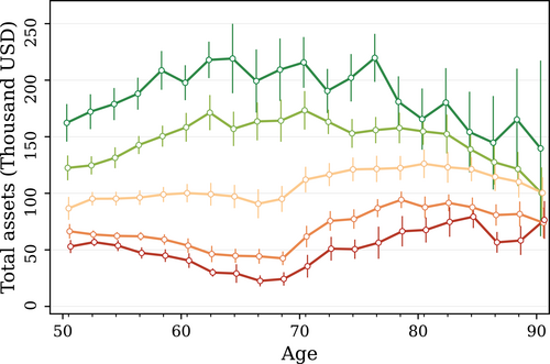
Median net total household wealth by self-reported health state. Pooled sample from HRS 1992–2014. Assets are adjusted for outliers, time, and cohort fixed effects. Colors indicate the health state: dark green is excellent while red is poor health. Error bars indicate 95% confidence intervals.
If individuals adjust their savings behavior based on their survival prospects, this could be either on the basis of objective (statistical) survival probabilities or subjective survival beliefs, which are also surveyed by the HRS. To assess how wealth correlates with survival beliefs, we regress net total wealth on an indicator of whether an individual believes to have above-median survival chances compared to other respondents of the same age, race, and sex. Table 1 shows a positive correlation between having above-median beliefs and being wealthier.4 The positive relationship also holds when additionally controlling for education and couple status.5 Other empirical studies corroborate the existence of the life expectancy/savings channel and suggest a causal link. For instance, Heimer, Myrseth, and Schoenle (2019) administer a novel survey and estimate that greater survival optimism correlates with higher savings rates, not only after controlling for standard demographic characteristics such as education, marital status, and income, but also financial literacy and risk tolerance.
|
Dep. Variable: Net Total Wealth (Inverse Hyperbolic Sine Transformation) |
||||||
|---|---|---|---|---|---|---|
|
Men |
Women |
|||||
|
(1) |
(2) |
(3) |
(4) |
(5) |
(6) |
|
|
Above median SSB |
0.418 |
0.230 |
0.221 |
0.575 |
0.374 |
0.353 |
|
(0.045) |
(0.040) |
(0.039) |
(0.032) |
(0.029) |
(0.029) |
|
|
Age FE |
Yes |
Yes |
Yes |
Yes |
Yes |
Yes |
|
Education FE |
Yes |
Yes |
Yes |
Yes |
||
|
Couple FE |
Yes |
Yes |
||||
|
Observations |
54,212 |
54,212 |
54,212 |
70,537 |
70,537 |
70,537 |
- Note: The table shows the results of regressing net total wealth (after an inverse hyperbolic sign transformation) on an indicator of above-median survival beliefs compared to individuals of the same age, race, and sex. The regression includes fully interacted fixed effects as indicated. Nonblack population. Clustered standard errors in parentheses.
Another prediction of the life expectancy/savings channel is that individuals who receive a bad health shock, that is, a plausible decrease in life expectancy, should exhibit lower asset growth. Table 2 reports the results from regressing the 2-year change in net total wealth (again using an inverse hyperbolic sine transformation) on a negative health shock defined as an indicator for a deterioration in self-reported health between survey waves. As column 1 shows, men who experience a negative health shock decumulate their assets more compared to men of the same race, age, and initial health who do not. Column 2 additionally controls for education, while columns 3–4 show the corresponding results for women. A negative health shock is associated with a faster decumulation (or slower accumulation) of assets in all specifications. More details are given in the Supplemental Appendix to the working paper (Foltyn and Olsson (2024)) (henceforth referred to as the Supplemental Appendix); see Section A.5.2.6
|
Dep. Variable: Relative Change in Net Total Wealth |
||||
|---|---|---|---|---|
|
Men |
Women |
|||
|
(1) |
(2) |
(3) |
(4) |
|
|
Negative health shock |
−0.149 |
−0.130 |
−0.134 |
−0.115 |
|
(0.023) |
(0.023) |
(0.018) |
(0.018) |
|
|
Age FE |
Yes |
Yes |
Yes |
Yes |
|
Health FE |
Yes |
Yes |
Yes |
Yes |
|
Education FE |
Yes |
Yes |
||
|
Observations |
61,528 |
61,528 |
80,615 |
80,615 |
- Note: The table shows the results of regressing changes in net total wealth (after an inverse hyperbolic sign transformation) on an indicator for a deterioration in self-reported health between two consecutive survey waves. The regression includes fully interacted fixed effects as indicated. Nonblack population. Clustered standard errors in parentheses.
While these results are indicative, a recent study by Kvaerner (2022) using the plausibly exogenous timing of cancer diagnoses shows that news about a bad health shock increases the probability of an immediate inter vivos transfer, suggesting a causal link between survival prospects and wealth decumulation. Thus, if a decrease in life expectancy increases own consumption and/or increases the probability of inter vivos transfers is an open question, and one interpretation of inter vivos transfers from the giver's perspective is to view them as “consumption of gift-giving.” While both inter vivos transfers and own consumption show up as a decumulation of assets and thereby affect the health-wealth gradient in older ages in the same way, they have different implications for wealth among the younger receiving generation, and thus for the wealth distribution. Our structural model does not allow for inter vivos transfers, and consequently, leaves this question open for future research.
2.3 Objective health and survival probabilities
In this paper, we examine the effect of heterogeneity in survival expectancy on savings behavior and its implications for wealth inequality through the lens of a structural model. Therefore, we need to formulate heterogeneity in survival expectations, both objective and subjective, in a way that can be used in such a model.
For our quantitative model, we use a Markov process for health transitions and survival at an annual frequency. We estimate this Markov process as described in Foltyn and Olsson (2021). Conceptually, the method is a straightforward maximum likelihood estimator where the probability of observing the transitions in the data is maximized. We briefly summarize the method and estimation sample in the next few paragraphs.
Estimation sample
We exclude all observations with missing age, race, sex, or self-reported health, as well as individuals with only a single observation (since then we do not have any transition probability to estimate). We only consider individuals aged 50 or older.8 Furthermore, we restrict the sample to maximum age of 99 years at transition start (even though individuals can be older when we observe them in the end of a transition). This leaves us with 34,196 individuals and 219,539 observations in total. We estimate the health and objective (statistical) survival process separately for the subsamples of men/women and the black/nonblack population, since it is well known that the life expectancies for these groups follow very different trajectories.9 Table B.1 in the Supplemental Appendix shows descriptive statistics and the number of individuals and observations by subgroup.
Results
From these estimates, we construct a first-order Markov process defined on five health states and the absorbing state of death, which governs the objective health and survival probabilities. This process can be used to calculate objective life expectancies conditional on age, health, race, and sex. Not surprisingly, there is a substantial health gradient in life expectancy. For example, for a 70-year-old nonblack man in excellent health, the predicted probability of surviving an additional 10 years is approximately 75%, while the probability is just around 35% if instead starting out in poor health. For a brief overview of the results, see the Supplemental Appendix, Section B.2.
It is important to note that even though the health and survival process is based on self-reported health—a subjective measure of how respondents perceive their health state—the result from the estimation is an objective statistical life expectancy for each combination of race, sex, age, and health. Self-reported health can be thought of as letting the respondents themselves aggregate the multidimensional information about their health (that is potentially unobservable to the econometrician) into a single categorical variable, and the variable can also capture subjective perceptions of the respondent. The estimated Markov process maximizes the probability of observing the health transitions and survival in the data conditional on self-reported health, irrespective of why a particular health state was reported.
2.4 Expectation errors in survival probabilities
In the expectations survey module of the HRS, respondents are asked about the probability they assign to certain events. One of these questions is about the probability of surviving to a certain age, for example: “Using a number from 0 to 100, what do you think are the chances that you will live to be at least 100 years?”10
The exact target age depends on the respondent's age and survey wave. For instance, in 1995, respondents below the age of 70 were asked about the probability of living until the age of 80, while respondents above the age of 85 were asked about the target age of 100. In later surveys, individuals were asked about survival beliefs for up to two target ages.
Table 3 shows the number of individuals and observations (an observation being one elicited survival belief) by subgroup. The tabulated distribution of target ages shows that the questions about survival to age 75 or 85 are by far the most common, hence we focus on these two in the main text.
|
All |
Nonblack |
Black |
|||
|---|---|---|---|---|---|
|
Male |
Female |
Male |
Female |
||
|
Sample size |
|||||
|
N. of individuals |
32,590 |
12,073 |
14,884 |
2274 |
3359 |
|
N. of observations |
252,299 |
92,013 |
120,481 |
14,914 |
24,891 |
|
Avg. observations/indiv. |
7.7 |
7.6 |
8.1 |
6.6 |
7.4 |
|
Forecast horizon (years) |
|||||
|
Min. |
10.0 |
10.0 |
10.0 |
10.0 |
10.0 |
|
Mean |
19.4 |
19.5 |
19.2 |
20.2 |
19.8 |
|
Max. |
39.0 |
35.0 |
39.0 |
35.0 |
35.0 |
|
Target age distribution |
|||||
|
Age 75 |
37.2% |
37.7% |
36.3% |
41.0% |
39.5% |
|
Age 80 |
16.3% |
16.3% |
16.4% |
15.3% |
16.1% |
|
Age 85 |
35.1% |
35.6% |
34.4% |
37.1% |
36.2% |
|
Age 90 |
5.6% |
5.3% |
6.1% |
3.7% |
4.3% |
|
Age 95 |
3.9% |
3.5% |
4.5% |
2.0% |
2.6% |
|
Age 100 |
2.0% |
1.7% |
2.4% |
0.9% |
1.3% |
- Note: Mean forecast horizon and distribution over target ages are weighted using HRS sample weights.
Using these elicited beliefs, we compare the average probability that individuals of a certain age assign to survival until a given target age to the probability according to official life tables. As can be seen in Figure 2, there is a systematic error along the age gradient: younger individuals on average tend to underestimate, while older individuals tend to overestimate their survival probability as compared to objective life table estimates.11
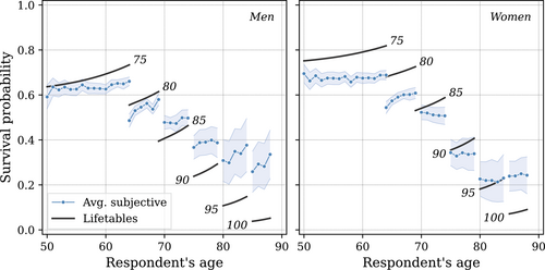
Objective versus subjective survival probabilities by age and sex (controlling for year and cohort fixed effects). The number next to the black line indicates target age. The blue line shows (weighted) average expectation in the nonblack population. Only age bins with at least 50 observations are shown.
This age-dependent error is a stylized fact in the literature on survival expectations (see, e.g., Ludwig and Zimper (2013), Groneck, Ludwig, and Zimper (2016), Heimer, Myrseth, and Schoenle (2019) and the references therein). The pattern has been used to, for example, improve the fit of the asset profile of the canonical life-cycle model with the data: due to underestimation early in life, young agents do not accumulate as much wealth, while overestimation in later years dampens the rate at which assets are decumulated.
Since our estimator conditions on health, race, and sex, we can go one step further and document survival belief differences along these dimensions. Figure 3 shows these expectation errors among respondents who have answered the question about their perceived probability of survival until target ages 75 and 85. The first observation is the striking positive correlation between subjective self-reported survival probability and the predicted (objective) survival probability, which means that subjective beliefs are informative. This is in line with the consensus in the literature, which finds that subjective beliefs are highly correlated with objective survival probabilities and serve as predictors of mortality, and that expectations are updated in the event of health shocks (Smith, Taylor, and Sloan (2001), Hurd and McGarry (2002), Gan, Hurd, and McFadden (2005)).
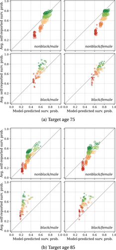
Elicited beliefs about survival versus estimated objective (statistical) survival probabilities. Each bubble represents the average for a race/sex/age/health group. The x-axis shows the model-predicted (objective) survival probability to the indicated target age. The y-axis shows the average self-reported survival probability for that group. Colors indicate the health state: dark green is excellent while red is poor health. The size indicates the number of observations in each cell. We exclude cells with less than 20 observations.
The second observation is the systematic steepness bias in beliefs over the health gradient. As was shown in Figure 2, on average individuals underestimate their probability of survival until the age of 75. Looking at Figure 3a, and focusing on nonblack males, it is clear that it is mainly individuals in bad health who are underestimating their survival probability, while individuals in excellent health are on average reasonably close to their objective survival probability.
Figure 3b shows expectation errors for target age 85. Again, individuals in bad health underestimate their survival probability more than those in good health, even though on average the expectations are more upward biased for this target age. Figure C.2 in the Supplemental Appendix shows the corresponding graphs for target age 95. The figure illustrates that for those higher ages individuals in bad health have beliefs closer to their objective probability, while individuals in good or excellent health are severely overestimating their survival chances. In the Supplemental Appendix, Section C.3, we additionally disaggregate the expectation errors by education. The overall picture remains unchanged.
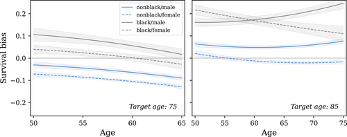
Survival bias by race, sex, and age. The graph shows the predicted from equation (2). A positive bias of 0.1 indicates that the group is overestimating their survival probability by 10 percentage points. Error bars indicate 95% confidence intervals.
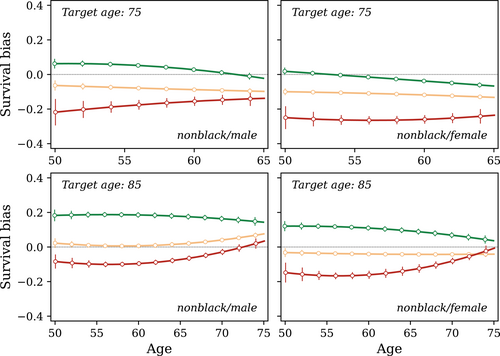
Survival bias by sex, age, and self-reported health for the nonblack population. The graph shows the predicted from equation (3). A positive bias of 0.1 indicates that the group is overestimating their survival probability by 10 percentage points. Colors indicate the health state: dark green is excellent while red is poor health. Error bars indicate 95% confidence intervals.
In a related paper, Grevenbrock et al. (2021) estimate survival based on several additional characteristics besides self-reported health, age, and sex, such as smoking and drinking behavior, and chronic diseases. Grouping individuals based on their estimated objective survival probability, they find that individuals with low objective survival probability in general overestimate, while individuals with high objective probability underestimate their survival probabilities; in other words, at a first glance the reverse pattern compared to what we find. However, there are two reasons for why our results are not directly comparable. First, they use a different estimation strategy for objective survival probabilities. Second, and more important, the grouping of individuals is different. We group based on age, sex, race, and self-reported health, which is the level of heterogeneity in our economic model (and thus, for our purposes, the most appropriate one) and show that, conditional on age, sex, and race, individuals with lower survival probabilities (poorer health) tend to underpredict their survival. Conversely, Grevenbrock et al. (2021) show that, when considering differences in survival due to age or permanent characteristics such as sex or race, groups with lower survival rates tend to overpredict their survival. For a more comprehensive discussion, see the Supplemental Appendix, Section C.5.
More generally, the finding that individuals with high life expectancy display an upward bias in their survival beliefs is in line with evidence about forecast errors in other domains. For example, Rozsypal and Schlafmann (2023) document that people in the upper part of the income distribution overestimate their future income growth while the opposite is true for lower-income households.
To summarize, we stress two observations: first, subjective beliefs are informative and correlated with objective probabilities. Second, subjective beliefs are biased. Subjective probabilities overestimate the health/survival gradient, with individuals in bad health underestimating their survival probability relative to individuals in good health. Hence, there is a systematic bias both along the age and health dimensions.
2.5 Estimation of the subjective life expectancy process
In this section, we use the health transitions estimated in Foltyn and Olsson (2021) as a basis for estimating a different set of parameters that govern subjective survival beliefs. The difference between objective probabilities and subjective beliefs could arise due to erroneous beliefs about survival conditional on health, erroneous beliefs about the health process, or a combination of the two. Without further information, we cannot distinguish between those alternatives, and the HRS does not elicit any beliefs about future health states. To keep the model reasonably parsimonious, we take as given the parameters controlling health-to-health transitions conditional on survival and estimate a different set of survival probabilities to capture the elicited beliefs.
We take an agnostic approach as to why the erroneous beliefs arise. In the literature, various mechanisms have been proposed, such as Choquet Bayesian learning models of survival beliefs, which allow for likelihood insensitivity (Ludwig and Zimper (2013), Groneck, Ludwig, and Zimper (2016)) and, closely related, age dependent cognitive weakness and relative optimism (Grevenbrock et al. (2021)) as well as overweighting the likelihood of rare events (Heimer, Myrseth, and Schoenle (2019)).
Estimation sample
We use all target ages from Table 3 for the estimation of the subjective life expectancy process. In the main paper, we present the results for nonblack men, as these are later incorporated into our quantitative model.
Results
The estimated subjective survival beliefs for nonblack men are shown in pink in Figure 6, juxtaposing the objective survival probabilities estimated in Foltyn and Olsson (2021) in blue. As can be seen, the subjective belief about survival in health state excellent or very good is almost 100% for all ages. This does not mean that individuals in those health states believe that they will live forever. Rather they believe that death is necessarily preceded by a deterioration in health.
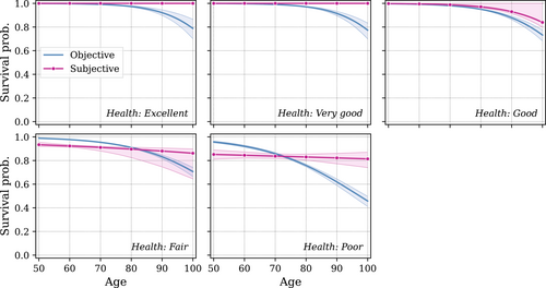
One-year objective and subjective survival probabilities by health state for nonblack men (model estimates). Shaded areas indicate 95% confidence intervals. For each bootstrapped sample, we reestimate the objective health process.
Figure 7 summarizes the results, showing the life expectancy by age and health state using the objective and the subjective survival process. At all ages, the difference in life expectancy between the best and the worst health state is larger when using subjective life expectancies. The divergence between objective and subjective life expectancies is particularly large for men in bad health, who substantially underestimate survival at younger ages. Conversely, individuals in all health states overestimate their chances of survival late in life. Figure C.8 in the Supplemental Appendix plots the objective and subjective life expectancy for the remaining demographic groups, which exhibit very similar patterns.
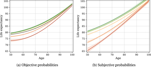
Life expectancy by age and health for nonblack men. Colors indicate the health state: dark green is excellent while red is poor health. In panel 7a, the black line depicts the weighted population average. Shaded areas indicate 95% confidence intervals.
Figure C.9 in the Supplemental Appendix plots the model-predicted subjective survival probabilities against their data counterparts, showing that both sets of moments are well aligned.
3 Economic model
In this section, we describe the overlapping-generations model used to quantify the implications of survival heterogeneity. Time is discrete and each period corresponds to one year. Agents derive utility from consumption and face idiosyncratic risk in the form of shocks to their labor income, medical expenditures, health and survival, as well as stochastic bequests from their parents. Markets are incomplete as agents can only save in a riskless asset while borrowing is not permitted.
3.1 The agent's problem
There is a unit mass of individuals distributed across cohorts according to the ergodic distribution implied by the transition matrix of survival probabilities. An individual of age and health has a one-period survival probability to age given by , with in the terminal period.13
Individuals are assumed to be working for the first years of their life and exogenously retire in the period in which they attain age . While working, they are hit by persistent and transitory labor productivity shocks. During retirement, individuals receive social security retirement benefits, which depend on their last persistent labor productivity in working age.
Bequests are modeled via probabilistic intergenerational links along the lines of Straub (2019) so that children with higher lifetime income are more likely to have income-rich parents, and thus expect to receive higher bequests.
Retirement
Working age
3.2 Technology
The production side of the model is standard. Competitive firms employ labor and capital hired from households to produce a homogeneous final good, which is used for both consumption and investment. The aggregate production function is assumed to be Cobb–Douglas, . Capital depreciates at the rate .
3.3 Government
We assume that the government runs a PAYGO social security system that has to balance in each period, and that transfers as well as any remaining (wasteful) government expenditures have to be fully financed by income and inheritance taxes. We first describe the social security system and thereafter the general government budget.
Social security system
Government budget
The government needs to finance lump-sum transfers ξ to households defined in (10). We denote the aggregate transfers by Ξ and provide details on how these are computed in the Supplemental Appendix, Section D.3.1. Additionally, the government finances nondiscretionary expenditures that amount to a constant fraction g of output, .
We assume that the progressivity parameter τ in (14) is fixed, and we pin down λ such that the government budget is balanced in each period, that is, .
3.4 Equilibrium
The equilibrium definition is mostly standard and can be found in the Supplemental Appendix, Section D.4. The one noteworthy addition is that we require that for each cohort, after-tax estates left by parents are consistent with the bequests expected and received by children given the stochastic intergenerational links. This introduces computational complications, which we discuss in the Supplemental Appendix, Section H.
4 Calibration
4.1 Preferences
We assume log preferences, that is, , and thus . The common discount factor is set to obtain a capital-to-output ratio of 3.0 in the scenario with subjective survival beliefs. In our benchmark calibration, we shut down the warm-glow bequest motive by setting , and hence all bequests are accidental. We discuss alternative scenarios in Section 5.4.
4.2 Externally calibrated parameters
Demographics
Agents are assumed to enter the economy at age 20, which corresponds to model age 1, and retire at the age of 65, implying that . The maximum attainable age is 109, and hence we let .15
Earnings
The age-health profile for labor earnings is estimated for nonblack men aged 20 to 65 using PSID data (PSID (2023)). Not surprisingly, there is a strong health gradient. This is partly driven by lower wages conditional on working, and partly by a larger fraction of individuals in bad health not working at all. Since we abstract from the labor supply decision, our estimates of the age-health earnings profile captures both margins. More details can be found in the Supplemental Appendix, Section E.3.
Medical expenditures
Following French and Jones (2004), De Nardi, French, and Jones (2010), we estimate the medical expenditure shocks from the out-of-pocket medical expenses reported at biennial frequency in the HRS for the sample of nonblack men aged 50 and above. Since the HRS includes hardly any individuals below the age of 50, we assume that agents do not face any out-of-pocket medical costs at these ages.
For the purpose of including medical expenditure shocks in the OLG model, we discretize the persistent component (15) using the Rouwenhorst procedure with seven states, and we discretize the transitory component (16) into five possible realizations.
Bequests
We assume that estates are tax exempt up to the amount and subject to a proportional tax thereafter. We set so that in equilibrium 2% of estates are subject to estate taxes, while is set to 30%.16 The intergenerational income quintile transition matrix used to link parents to children is taken from Chetty et al. (2014, Table II) and reproduced in Table D.1 in the Supplemental Appendix. Lastly, we allow the probability to receive a bequest conditional on parental death to differ by income quintile. To this end, we use the Survey of Consumer Finances (SCF) waves 1998–2007 and compute the fraction of respondents aged 60–70 who report having ever received an inheritance by each income quintile, which gives the probabilities 20.5%, 25.2%, 27.4%, 33.3%, and 40.4% for the lowest to highest quintile.
Remaining externally calibrated parameters
The remaining parameters are listed in Table 4. The bend points and the contribution and benefit base are reported in US dollars to facilitate the interpretation. The value for the consumption floor is similar to the levels used by De Nardi, French, and Jones (2010) or Palumbo (1999).
|
Parameter |
Description |
Value |
Source |
|---|---|---|---|
|
Production technology parameters |
|||
|
αk |
Capital share |
36% |
|
|
δk |
Depreciation rate |
9.6% |
|
|
A |
Total factor productivity |
0.896 |
Fixes equilibrium wages at unity |
|
Social security |
|||
|
ρ1 |
Replacement rate bracket 1 |
90% |
2000 SS rules |
|
ρ2 |
Replacement rate bracket 2 |
32% |
2000 SS rules |
|
ρ3 |
Replacement rate bracket 3 |
15% |
2000 SS rules |
|
|
Bendpoint 1 |
$6384 |
2000 SS rules |
|
|
Bendpoint 2 |
$38,424 |
2000 SS rules |
|
|
Contribution and benefit base (CBB) |
$76,200 |
2000 SS rules |
|
|
Consumption floor |
$2325 |
5% of average annual earnings |
|
Government budget |
|||
|
g |
Gov. spending (share of GDP) |
6% |
Brinca Holter, Krusell, and Malafry (2016) |
|
τ |
Tax progressivity |
0.137 |
|
|
τb |
Marginal tax on estates |
30% |
Authors' approximation |
4.3 Health and survival process
We use the processes for health transitions and survival probabilities described in Section 2.3 (health transitions and objective survival probabilities) and Section 2.5 (subjective survival probabilities) for nonblack men. Agents enter the model at the age of 20, but the health and survival processes we estimate based on the HRS data starts at the age of 50. We therefore estimate a health process for the ages 20 to 50 using PSID data. We use data from the years 1984 to 2019 and the subsample of nonblack male household heads, and assume that survival is certain during this age span (further details can be found in the Supplemental Appendix, Section E.1). From the age of 50, we use our estimated process based on the HRS data, and agents start facing a positive probability of death. The resulting cohort sizes and distribution of health states are shown in Figure E.2 in the Supplemental Appendix.
While the model is solved with five health states, in what follows we report results only for the best, middle, and worst health states to reduce visual clutter.
5 Results
We solve the model under three distinct assumptions about health heterogeneity and survival expectations:
- (i) No health heterogeneity (NHH): In this scenario, all agents of the same age face the same earnings profile, the same medical expenditure risk, and the same survival risk. We eliminate health heterogeneity and use the average survival rates (depicted by the black line in Figure 7a), an average earnings profile, and the average medical expenditure process. The probability of receiving an inheritance and the amount received are also averaged across health.17
- (ii) Objective survival heterogeneity (OSH): In the second scenario, we use the objective process for health transitions and survival probabilities described in Section 2.3. In this case, individuals are perfectly informed about their true survival probability conditional on health and age. Medical expenditures and labor earnings are allowed to differ by age and health.
- (iii) Subjective survival heterogeneity (SSH): In the third scenario, agents conversely form beliefs and act according to the subjective survival process estimated in Section 2.5. However, this subjective process does not correspond to the true survival process, which we use when simulating the model.
In the remainder of this section, we first contrast the effective discount rates that arise in the objective versus subjective survival belief scenarios. These are important drivers of savings behavior, which we discuss next. We then turn to the implications for wealth accumulation across health and also briefly discuss general equilibrium effects, which are mostly unchanged across all three scenarios. In our benchmark calibration, there is no warm-glow bequest motive, but lastly, we analyze how (subjective) survival heterogeneity interacts with an active bequest motive.
5.1 Effective discount rates
An individual's effective discount rate (determined by the common discount factor β and the survival probabilities) in the model is time varying and depends on the horizon. Following a bad health shock, the discount rate immediately rises since it implies a shorter expected life span, while the opposite happens in the event of a good health shock.
Figure 8 plots the effective average discount rates for different time horizons. As can be seen, the effective discount rate varies substantially in the population. Using the subjective probabilities, the 1-year horizon discount rate for a 50-year-old agent in good health is observationally equivalent to (since the 1-year ahead survival for this agent is perceived to be almost certain), while the 1-year horizon discount rate for an equally old agent in bad health is almost 20%. This gap shrinks at longer horizons but is still 7.9 percentage points at a 10-year horizon. For 70-year-old agents in worst versus best health state, the difference at the 10-year horizon is 9.5 percentage points.
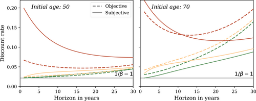
Effective discount rate (geometric average) as a function of initial (current) age (50 or 70), forecast horizon (on the x-axis), and objective or subjective survival probabilities (dashed vs. solid lines). Colors indicate the health state: dark green is excellent while red is poor health. The black line represents the discount rate net of any survival effect.
The magnitude of the dispersion of subjective discount rates is consistent with the findings by Calvet et al. (2021) who estimate the cross-sectional distribution of time preference rates based on Swedish micro data, assuming a common survival probability conditional on age for all agents. They estimate the standard deviation of the time preference rate to be 7.0 percentage points around a mean of 5.2%.
The magnitude of the differences between discount rates based on subjective beliefs and objective survival probabilities across health states are well in line with the discount factor heterogeneity estimated by De Nardi, Pashchenko, and Porapakkarm (2017). In a model with rational survival expectations, they find that individuals in bad health on average have a higher discount rate (i.e., are more impatient). Our results show that the difference between the subjective and objective discount rate is larger for individuals in bad health, and the magnitude of these differences is consistent with their estimates (see the Supplemental Appendix, Section F.1 for details).
The pattern of subjective and objective discount rates are also consistent with an average downward-sloping discount rate along the age gradient, as found by Kureishi et al. (2021). Netting out the average objective (statistical) survival probability at all ages, the belief bias in survival probabilities gives rise to a downward sloping residual discount rate, since older people on average display an upward bias in their beliefs about survival compared to the young (see Figure 2).
5.2 Effect on savings behavior
The effect of subjective survival beliefs on savings varies depending on age and health. Working-age individuals in good health have on average higher earnings (see the earnings profiles in Figure E.3 in the Supplemental Appendix) and slightly higher consumption. The savings rate in this group is thus primarily driven by the desire to smooth consumption over the life cycle (which includes more years in retirement due to higher life expectancy) and a precautionary savings motive (to insure against adverse health shocks). Whether they act according to subjective or objective survival probabilities has little impact since agents in good health just prior to retirement do not have a very pronounced survival bias (see Figure 5). Working-age individuals in poor health, on the other hand, save substantially less when endowed with subjective survival beliefs since these agents underestimate their survival prospects.
These differences in savings behavior are illustrated in Figure 9. For selected health states, the hatched bars show the differences in total savings rates for the model with objective survival heterogeneity compared to the model with no health heterogeneity (NHH) disaggregated by deciles of the cash-at-hand distribution. The bars in lighter color show the additional effect of imposing subjective beliefs. In these graphs, we define the total savings rate as the fraction of cash-at-hand, that is, beginning-of-period assets plus current income, which the individual saves for the next period.18
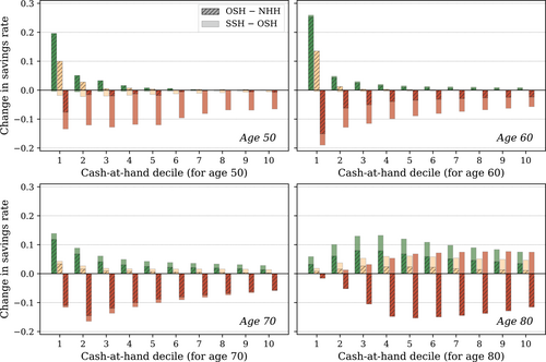
Differences in savings rates (defined as the fraction of current cash-at-hand the agent saves for the next period). The hatched bars show the difference between the objective survival heterogeneity and no health heterogeneity models conditional on age, health, and cash-at-hand decile. The lighter bars show the additional effect of imposing subjective survival beliefs. Colors indicate health state: green is excellent while red is poor health.
As can be seen, the 50-year-olds in poor health save substantially less across the cash-at-hand distribution, and the difference is mainly driven by the bias in survival beliefs. When acting according to subjective beliefs, 50-year-old agents in poor health severely underestimate their remaining life span and, therefore, save approximately 10 percentage points less than in the no-health heterogeneity model.
The same pattern can be seen in the graph for 70-year-olds, even though the additional effect from adding the subjective beliefs is slightly weaker (still focusing on the agents in poor health). The reason for this can be found in Figure 5: at the age of 70, the subjective survival beliefs of the agents in bad health are close to the objective probabilities. Moreover, at the age of 70, the effect of the subjective beliefs starts showing up more substantially for agents in good health as indicated by the lighter green parts of the green bars.
As can be seen from the graph of 80-year-olds, at higher ages the general optimism dominates. The addition of subjective beliefs at this age increases the savings rates for agents both in bad and good health.
5.3 Effect on wealth accumulation
Figure 10 shows the resulting life-cycle profiles for wealth for the three different scenarios: no health heterogeneity (NHH), objective survival heterogeneity (OSH), and subjective survival heterogeneity (SSH). We average out all states other than assets, health, and age.
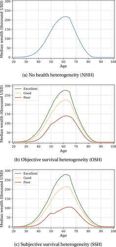
Life-cycle profiles for median wealth for different scenarios. Colors indicate the health state: dark green is excellent while red is poor health. In panel 10a, there is no health heterogeneity.
For all three models, the life-cycle profile for wealth peaks at the age of 64, which is the last year before retirement. When agents enter retirement, they start drawing down their wealth and the median individual who survives until the age of 90 has drawn down all of his savings (remember that all individuals receive retirement benefits and, if needed, government transfers, so they are not risking zero consumption).
The profile for the OSH model illustrates that agents in bad health accumulate less wealth than agents in good or excellent health when endowed with objective beliefs about survival. It should be noted that the mass of agents in bad health is not static but consists of individuals who have been in bad health for many periods, as well as individuals who recently drew a bad health shock.
Next, the profile for the SSH model shows that the difference in wealth between agents in best and worst health increases when the agents act according to their subjective beliefs. Note also that compared to the NHH and OSH models, the asset holdings at very high ages increase slightly, since old agents, on average, overestimate their remaining lifespan.
In the SSH model, the median wealth among 50–54 year olds in poor health is 36% of the median wealth held by those in excellent health of the same age. This health-wealth gap is very close to what we observe in the HRS (where the corresponding figure for nonblack males in the age group 50–54 is 34%).19 A substantial part of this gap is due to biased survival beliefs: in the OSH model, where agents have rational expectations about their survival, the corresponding figure is 49%. Thus, the biases in survival beliefs explain approximately a fifth of the health-wealth gap in this age group.20
General equilibrium effects and economywide inequality
We now turn to economy-wide wealth inequality and general equilibrium effects. The first model in Table 5 (SSH-GE) shows the Gini coefficient for wealth (0.70) from the benchmark model with subjective beliefs in general equilibrium. The second model (OSH-PE-1) is a partial equilibrium exercise in which we keep aggregate variables from the SSH-GE scenario (interest rate, wage rate, taxes, and distribution of bequests received) but let agents act according to objective survival probabilities. In the OSH-PE-1 model, the Gini coefficient for wealth decreases slightly to 0.69. With objective survival beliefs, agents in the age group around 55–65 no longer have a downward bias in expected longevity and, therefore, higher incentives to save. This effect is strongest among the agents in poor health with low asset holdings, and thus the result is fewer poor individuals close to retirement.
|
Beliefs |
GE |
r |
w |
λ |
Bequests |
Gini |
|
|---|---|---|---|---|---|---|---|
|
Subjective survival probabilities |
|||||||
|
SSH-GE |
subjective |
yes |
2.37% |
1.0000 |
0.9222 |
SSH |
0.701 |
|
Objective survival probabilities |
|||||||
|
OSH-PE-1 |
objective |
no |
2.37% |
1.0000 |
0.9222 |
SSH |
0.694 |
|
OSH-PE-2 |
objective |
no |
2.19% |
1.0000 |
0.9222 |
SSH |
0.701 |
|
OSH-PE-3 |
objective |
no |
2.19% |
1.0086 |
0.9222 |
SSH |
0.700 |
|
OSH-PE-4 |
objective |
no |
2.19% |
1.0086 |
0.9233 |
SSH |
0.700 |
|
OSH-GE |
objective |
yes |
2.19% |
1.0086 |
0.9233 |
OSH |
0.702 |
|
No health heterogeneity |
|||||||
|
NHH-GE |
average |
yes |
2.30% |
1.0032 |
0.9189 |
NHH |
0.715 |
- Note: Gini coefficient for different model scenarios in general and partial equilibrium (as indicated by column “GE”). Row OSH-PE-1 imposes the same aggregates as SSH-GE but introduces objective survival beliefs. Rows OSH-PE-2 to OSH-PE-4 additionally incrementally impose the equilibrium interest rate, wages, and tax rate from the OSH model. The “Bequests” columns indicate which equilibrium bequests were used.
The models labeled OSH-PE-2 to 4 incrementally replace the aggregate variables with the ones from the general equilibrium model with objective beliefs. The equilibrium interest rate with objective survival beliefs is lower than with subjective beliefs. Removing the average downward survival bias among the agents close to retirement (which is when life-cycle assets peak) results in higher demand for assets in the model with objective beliefs. For the capital market to clear, the interest rate needs to fall. The OSH-PE-2 model uses the lower interest rate, but otherwise the same setting as the OSH-PE-1. The Gini coefficient increases slightly from 0.69 to 0.70. There are two reasons. First, with a lower interest rate agents save less in general. Since agents with low productivity and bad health receive lower bequests, the decrease in savings have a relatively stronger effect on their total wealth.21 Second, a lower interest rate increases frontloading of consumption over the life cycle and, therefore, results in slightly more poor elderly in the economy.
As the results from the OSH-PE-3, OSH-PE-4, and OSH-GE models show, the shifts of wage rate, taxes, and distribution of bequests have virtually no effect on the economy-wide Gini coefficient for wealth.
The last row in Table 5 shows the general equilibrium results from the model with no health heterogeneity. The Gini coefficient for wealth is slightly higher than in any of the models with health heterogeneity. The driver of this is an increased number of large accidental bequests. The largest amounts bequethed stem from deaths in relatively young ages (between ages 50 and 65). In a model with no health heterogeneity, these deaths are equally likely to happen to agents in the top of the asset distribution as to agents in the bottom. With health-dependent survival on the other hand, it is more likely that deaths in relatively young ages happen to agents in poor health, who are on average poorer. Thus, the lack of health heterogeneity gives rise to larger bequests, which in turn gives rise to slightly larger wealth inequality.
5.4 A model with an active bequest motive
There are many drivers of savings that could vary across health but are not included in our model: the existence of (employer-tied) health or life insurance, human capital investment, endogenous retirement decisions, portfolio composition, private pensions, and permanent characteristics such as patience, to name a few (see, for instance, De Nardi, French, and Jones (2010), Capatina (2015), or De Nardi, Pashchenko, and Porapakkarm (2017) for studies taking a broader perspective including several channels). These mechanisms could all add realism to the model and make the life-cycle profiles more in line with the data. One mechanism often introduced to capture the slow decumulation of asset in older ages is a warm-glow bequest motive. In this section, we therefore use a model calibration with an active bequest motive () to show how it interacts with (subjective) survival heterogeneity.
5.4.1 Calibration
Where applicable, we use the same calibration as in the main text. We determine the discount factor β, the preference parameters governing the bequest motive ( and ) and the estate tax exemption threshold using the method of simulated moments, that is, we minimize the weighted sum of squared distances between targeted and simulated moments from the model with subjective beliefs about survival.
We again target a capital-to-output ratio of 3 and that 2% of estates should be subject to estate taxes. Additionally, we try to match the old-age, life-cycle profile of assets. To this end, we use the median wealth levels at ages 60, 65, 70, 75, 80, and 85 observed in the HRS, relative to median wealth at age 55. We choose this approach as it is quantitatively not possible to match wealth in levels and at the same time impose a capital-output-ratio of 3 in a model with productive capital as the only asset (after all, most of the wealth in the data is held in residential real estate). The capital-to-output ratio and the fraction of estates subject to estate tax are perfectly matched, while the asset holdings by age and their data counterparts are shown in Table G.1 in the Supplemental Appendix. Some aspects of our model are too simplistic to match the data moments exactly. For example, because we impose an exogenous retirement age of 65, the life-cycle profile of assets peaks exactly at this age, whereas this is not the case in the data.
The estimated parameters are listed in Table 6. As the table shows, the bequest luxury shifter is small. The reason is that we try to match the median asset holdings late in life. If bequests were a luxury good, the median asset level would fall quickly toward zero.
|
Parameter |
Description |
Value |
|---|---|---|
|
Model with bequest |
||
|
β |
Discount factor |
0.942 |
|
ϕ1 |
Bequest weight |
11.157 |
|
ϕ2 |
Bequest shifter |
0.001 |
|
χb |
Estate tax exemption |
18.333 |
5.4.2 Results
Cross-section and life cycle
Figure 11 shows the life-cycle profiles for the scenarios with objective survival heterogeneity (OSH) and subjective survival heterogeneity (SSH). Overall, due to the bequest motive, older agents do not decumulate their wealth, and the resulting median asset profile is more in line with the data in both scenarios. Before retirement, agents in excellent health have more wealth than agents in worse health. The main reason for this is the higher labor income of the former group.
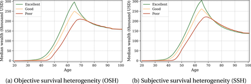
Median life-cycle profiles for wealth, model with an active bequest motive.
However, the health-wealth gradient is substantially smaller prior to retirement than in the baseline calibration without a bequest motive (compare to Figure 10), and is even reversed after the age of 75, with agents in poor health being richer. This shows that the effect of combining survival heterogeneity with a bequest motive of this type is not entirely straightforward. The expected utility from leaving a bequest is not only a function of the amount expected to be handed over to the descendants, but also of the survival probability: agents with low (objective or subjective) survival prospects put more weight on the bequest motive. Hence, there are two effects from lower life expectancy that work in opposite directions: a shorter expected life span makes agents want to save less for their own consumption in old age, but a stronger bequest motive induces them to save more. The net effect varies depending on the calibration of bequest parameters, but the second mechanism is always present with a warm-glow bequest motive of this type: a shorter life span makes agents want to save more to leave bequests.22
Thus, in both the OSH and the SSH scenario, the model misses the cross-sectional correlation between wealth and health in older ages that is present in the data. The slightly stronger reversal of the health-wealth gradient in the SSH model follows directly from the biases that amplify the health-survival belief gradient.
Note also that in very high ages, agents keep less assets in the SSH model than in the OHS model. Agents in the subjective belief model overestimate the probability of a long life and, therefore, put a lower weight on warm-glow bequests, resulting in lower savings.
Dynamic responses to health shocks
Next, we compare changes in wealth following negative health shocks in the data to their model counterparts. To this end, we regress the change in net total wealth (using an inverse hyperbolic sine transformation) on a negative health shock defined as an indicator for a deterioration in self-reported health between survey waves. We restrict the sample to ages 65 and above in order to focus on the part of the life cycle where life expectancy and bequest considerations are important drivers of savings. We simulate a panel of 100,000 agents and collapse the data to two-year frequency to replicate the biennial HRS.23 The changes in assets and health are defined analogously to the data, taking differences over 2-year periods.
The results in Table 7 show that the model with a bequest motive produces dynamic savings responses that are difficult to square with the data. The estimated savings response to a negative health shock in the model with an active bequest motive is effectively zero, whereas the model without an active bequest motive produces savings responses that are well in line with the data.
|
Dep. Variable: Relative Change in Net Total Wealth |
||||
|---|---|---|---|---|
|
Data |
Model |
|||
|
(1) |
(2) |
No bequest |
Bequest |
|
|
Negative health shock |
−0.116 |
−0.105 |
−0.1081 |
0.0001 |
|
(0.026) |
(0.026) |
(0.001) |
(0.000) |
|
|
Age FE |
Yes |
Yes |
Yes |
Yes |
|
Health FE |
Yes |
Yes |
Yes |
Yes |
|
Education FE |
Yes |
|||
|
Observations |
35,821 |
35,821 |
1,297,804 |
1,297,804 |
- Note: The table shows the results of regressing changes in net total wealth (after an inverse hyperbolic sign transformation) on an indicator for a deterioration in self-reported health between two consecutive survey waves. The regression includes fully interacted fixed effects as indicated. Columns 1 and 2 are the same as the first two columns in Table A.5 in the Supplemental Appendix. For the model columns, we use the SSH scenario where agents act according to their subjective beliefs. Sample restricted to nonblack males age 65 and above. Clustered standard errors in parentheses.
In sum, in a model with health heterogeneity, both the cross-sectional implications and the dynamic responses to health shocks make the model with a bequest motive calibrated to match median asset holdings in old age difficult to align with data. The relative strength of the different effects we point to in this section of course varies depending on calibration, but should be kept in mind when combining a warm-glow bequest motive with dynamically evolving expected longevity.
6 Conclusions
This paper explores how variation in objective and subjectively perceived life expectancy affects savings behavior of healthy and unhealthy people. Using HRS data, we show that there exists a within-cohort steepness bias in survival beliefs: individuals in bad health not only have a shorter expected life span, but are also relatively more downward biased about their survival chances, while individuals in good health, and thus with higher survival probability display a more upward bias. These systematic biases exacerbate the survival expectancy heterogeneity in the population.
The differences in beliefs about survival translate into time preference heterogeneity, and consequently, savings behavior. We show that biases in beliefs about survival can explain approximately one-fifth of the differences in accumulated wealth between those in excellent versus poor health, mostly because the latter group underestimates their life expectancy.
This paper ties into a strand of current research investigating preference heterogeneity and its importance for individual choices and aggregate outcomes. We provide an intuitively plausible and micro-founded source of heterogeneity: the perceived probability of surviving to future states of the world. Our quantification of this channel shows that life expectancy heterogeneity is important and should be included in the list of potential sources of heterogeneity that we need to consider in our analyses. Investigating the importance of the steepness bias for within-cohort differences in terms of portfolio allocations, demand for financial products, or retirement behavior is left for future research.


