Confidence Intervals for Projections of Partially Identified Parameters
Abstract
We propose a bootstrap-based calibrated projection procedure to build confidence intervals for single components and for smooth functions of a partially identified parameter vector in moment (in)equality models. The method controls asymptotic coverage uniformly over a large class of data generating processes. The extreme points of the calibrated projection confidence interval are obtained by extremizing the value of the function of interest subject to a proper relaxation of studentized sample analogs of the moment (in)equality conditions. The degree of relaxation, or critical level, is calibrated so that the function of θ, not θ itself, is uniformly asymptotically covered with prespecified probability. This calibration is based on repeatedly checking feasibility of linear programming problems, rendering it computationally attractive.
Nonetheless, the program defining an extreme point of the confidence interval is generally nonlinear and potentially intricate. We provide an algorithm, based on the response surface method for global optimization, that approximates the solution rapidly and accurately, and we establish its rate of convergence. The algorithm is of independent interest for optimization problems with simple objectives and complicated constraints. An empirical application estimating an entry game illustrates the usefulness of the method. Monte Carlo simulations confirm the accuracy of the solution algorithm, the good statistical as well as computational performance of calibrated projection (including in comparison to other methods), and the algorithm's potential to greatly accelerate computation of other confidence intervals.
1 Introduction
This paper provides novel confidence intervals for projections and smooth functions of a parameter vector  ,
,  , that is partially or point identified through a finite number of moment (in)equalities. In addition, we develop a new algorithm for computing these confidence intervals and, more generally, for solving optimization problems with “black box” constraints, and obtain its rate of convergence.

 aggregates violations of the sample analog of the moment (in)equalities and the critical value
  controls asymptotic coverage, often uniformly over a large class of data generating processes (DGPs). However, applied researchers are frequently interested in a specific component (or function) of θ, for example, the returns to education. Even if not, they may simply want to report separate confidence intervals for components of a vector, as is standard practice in other contexts. Thus, consider inference on the projection
  , where p is a known unit vector. To date, it is common to report as confidence set the corresponding projection of
  or the interval
 (1.1)
(1.1) -consistent estimator
  with limiting covariance matrix equal to the identity matrix, the usual 95% confidence interval for
  equals
  . Yet the analogy to
  would be projection of a 95% confidence ellipsoid, which with
  yields
  and a true coverage of essentially 1.
 calibrated so that the projection of
  covers
  (but not necessarily θ) with probability at least
  . As a confidence region for the true
  , one may report this projection, that is,
 (1.2)
(1.2) (1.3)
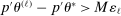
(1.3)Computationally, calibration of  is relatively attractive: We linearize all constraints around θ, so that coverage of
  can be calibrated by analyzing many linear programs. Nonetheless, computing the above objects is challenging in moderately high dimension. This brings us to our second contribution, namely, a general method to accurately and rapidly compute confidence intervals whose construction resembles (1.3). Additional applications within partial identification include projection of confidence regions defined in Chernozhukov, Hong, and Tamer (2007), Andrews and Soares (2010), or Andrews and Shi (2013), as well as (with minor tweaking; see Appendix B) the confidence interval proposed in Bugni, Canay, and Shi (2017, BCS henceforth) and further discussed later. In an application to a point identified setting, Freyberger and Reeves (2017, Supplement Section S.3) used our method to construct uniform confidence bands for an unknown function of interest under (nonparametric) shape restrictions. They benchmarked it against gridding and found it to be accurate at considerably improved speed. More generally, the method can be broadly used to compute confidence intervals for optimal values of optimization problems with estimated constraints.
Our algorithm (henceforth called E-A-M for Evaluation-Approximation-Maximization) is based on the response surface method; thus, it belongs to the family of expected improvement algorithms (see, e.g., Jones (2001), Jones, Schonlau, and Welch (1998), and references therein). Bull (2011) established convergence of an expected improvement algorithm for unconstrained optimization problems where the objective is a “black box” function. The rate of convergence that he derived depends on the smoothness of the black box objective function. We substantially extend his results to show convergence, at a slightly slower rate, of our similar algorithm for constrained optimization problems in which the constraints are sufficiently smooth “black box” functions. Extensive Monte Carlo experiments (see Appendix C and Section 5 of Kaido, Molinari, and Stoye (2017)) confirm that the E-A-M algorithm is fast and accurate.
Relation to Existing Literature. The main alternative inference procedure for projections—introduced in Romano and Shaikh (2008) and significantly advanced in BCS—is based on profiling out a test statistic. The classes of DGPs for which calibrated projection and the profiling-based method of BCS (BCS-profiling henceforth) can be shown to be uniformly valid are non-nested.1
Computationally, calibrated projection has the advantage that the bootstrap iterates over linear as opposed to nonlinear programming problems. While the “outer” optimization problems in (1.3) are potentially intricate, our algorithm is geared toward them. Monte Carlo simulations suggest that these two factors give calibrated projection a considerable computational edge over profiling, though profiling can also benefit from the E-A-M algorithm. Indeed, in Appendix C, we replicate the Monte Carlo experiment of BCS and find that adapting E-A-M to their method improves computation time by a factor of about 4, while switching to calibrated projection improves it by a further factor of about 17.
In an influential paper, Pakes, Porter, Ho, and Ishii (2011, PPHI henceforth) also used linearization but, subject to this approximation, directly bootstrapped the sample projection. This is valid only under stringent conditions.2 Other related articles that explicitly consider inference on projections include Beresteanu and Molinari (2008), Bontemps, Magnac, and Maurin (2012), Kaido (2016), and Kline and Tamer (2016). None of these establish uniform validity of confidence sets. Chen, Christensen, and Tamer (2018) established uniform validity of MCMC-based confidence intervals for projections, but aimed at covering the projection of the entire identified region  (defined later) and not just of the true θ. Gafarov, Meier, and Montiel-Olea (2016) used our insight in the context of set identified spatial VARs.
Regarding computation, previous implementations of projection-based inference (e.g., Ciliberto and Tamer (2009), Grieco (2014), Dickstein and Morales (2018)) reported the smallest and largest value of  among parameter values
  that were discovered using, for example, grid-search or simulated annealing with no cooling. This becomes computationally cumbersome as d increases because it typically requires a number of evaluation points that grows exponentially with d. In contrast, using a probabilistic model, our method iteratively draws evaluation points from regions that are considered highly relevant for finding the confidence interval's endpoint. In applications, this tends to substantially reduce the number of evaluation points.
Structure of the Paper. Section 2 sets up notation and describes our approach in detail, including computational implementation of the method and choice of tuning parameters. Section 3.1 establishes uniform asymptotic validity of  , and Section 3.2 shows that our algorithm converges at a specific rate which depends on the smoothness of the constraints. Section 4 reports the results of an empirical application that revisits the analysis in Kline and Tamer (2016, Section 8). Section 5 draws conclusions. The proof of convergence of our algorithm is in Appendix A. Appendix B shows that our algorithm can be used to compute BCS-profiling confidence intervals. Appendix C reports the results of Monte Carlo simulations comparing our proposed method with that of BCS. All other proofs, background material for our algorithm, and additional results are in the Supplemental Material (Kaido, Molinari, and Stoye (2019)).3
2 Detailed Explanation of the Method
2.1 Setup and Definition of 
 be a random vector with distribution P, let
  denote the parameter space, and let
  for
for  denote known measurable functions characterizing the model. The true parameter value θ is assumed to satisfy the moment inequality and equality restrictions
 (2.1)
(2.1) (2.2)
(2.2) is the set of parameter values in Θ satisfying (2.1)–(2.2). For a random sample
  of observations drawn from P, we write

 . The confidence interval in (1.3) then is
 (2.3)
(2.3) (2.4)
(2.4) . Henceforth, to simplify notation, we write
  for
for  . We also define
  moments, where
  for
for  . That is, we treat moment equality constraints as two opposing inequality constraints.
 that we specify below, define the asymptotic size of
  by4
by4
 (2.5)
(2.5) .
.2.2 Calibration of 
Calibration of  requires careful analysis of the moment restrictions' local behavior at each point in the identification region. This is because the extent of projection conservatism depends on (i) the asymptotic behavior of the sample moments entering the inequality restrictions, which can change discontinuously depending on whether they bind at θ or not, and (ii) the local geometry of the identification region at θ, that is, the shape of the constraint set formed by the moment restrictions. Features (i) and (ii) can be quite different at different points in
  , making uniform inference challenging. In particular, (ii) does not arise if one only considers inference for the entire parameter vector, and hence is a new challenge requiring new methods.
 and
and  . The projection of θ is covered when
 (2.6)
(2.6) and took λ to be the choice parameter; intuitively, this localizes around θ at rate
  . We then make the event smaller by adding the constraint
  , with
  and
and  a tuning parameter. We motivate this step later.
 . To ease computation, we approximate (2.6) by linear expansion in λ of the constraint set. For each j, add and subtract
  and apply the mean value theorem to obtain
 (2.7)
(2.7) is a normalized empirical process indexed by
  ,
,  is the gradient of the normalized moment,
  is the studentized population moment, and the mean value
  lies componentwise between θ and
  .5
.5 with a uniformly consistent (on compact sets) estimator,
  ,6 and the process
  with its simple nonparametric bootstrap analog,
  .7 Estimation of
  is more subtle because it enters (2.7) scaled by
  , so that a sample analog estimator will not do. However, this specific issue is well understood in the moment inequalities literature. Following Andrews and Soares (2010, AS henceforth) and others (Bugni (2010), Canay (2010), Stoye (2009)), we shrink this sample analog toward zero, leading to conservative (if any) distortion in the limit. Formally, we estimate
  by
by  , where
  is one of the Generalized Moment Selection (GMS henceforth) functions proposed by AS,

 is a user-specified thresholding sequence.8 In sum, we replace the random constraint set in (2.6) with the (bootstrap-based) random polyhedral set9
 (2.8)
(2.8) to be used in (2.4) then is
 (2.9)
(2.9) (2.10)
 denotes the law of the random set
  induced by the bootstrap sampling process, that is, by the distribution of
  conditional on the data. Expression (2.10) uses convexity of
  and reveals that the probability inside curly brackets can be assessed by repeatedly checking feasibility of a linear program.10 We describe in detail in Supplemental Material Appendix D.4 how we compute
  through a root-finding algorithm.
We conclude by motivating the “ρ-box constraint” in (2.6), which is a major novel contribution of this paper. The constraint induces conservative bias but has two fundamental benefits: First, it ensures that the linear approximation of the feasible set in (2.6) by (2.8) is used only in a neighborhood of θ, and therefore that it is uniformly accurate. More subtly, it ensures that coverage induced by a given c depends continuously on estimated parameters even in certain intricate cases. This renders calibrated projection valid in cases that other methods must exclude by assumption.11
2.3 Computation of  and of Similar Confidence Intervals
Projection-based methods as in (1.1) and (1.3) have nonlinear constraints involving a critical value which, in general, is an unknown function, with unknown gradient, of θ. Similar considerations often apply to critical values used to build confidence intervals for optimal values of optimization problems with estimated constraints. When the dimension of the parameter vector is large, directly solving optimization problems with such constraints can be expensive even if evaluating the critical value at each θ is cheap.
 (2.11)
 is an optimal solution of the problem and
  ,
,  as well as
  are fixed functions of θ. In our own application,
  and, for calibrated projection,
  .12
.12The key issue is that evaluating  is costly.13 Our algorithm does so at relatively few values of θ. Elsewhere, it approximates
  through a probabilistic model that gets updated as more values are computed. We use this model to determine the next evaluation point but report as tentative solution the best value of θ at which
  was computed, not a value at which it was merely approximated. Under reasonable conditions, the tentative optimal values converge to
  at a rate (relative to iterations of the algorithm) that is formally established in Section 3.2.
After drawing an initial set of evaluation points that we set to grow linearly with d, the algorithm has three steps called E, A, and M below.
Initialization: Draw randomly (uniformly) over Θ a set  of initial evaluation points. Evaluate
  for
for  . Initialize
  .
.
 and record the tentative optimal value

 .
. by a flexible auxiliary model. We use a Gaussian-process regression model (or kriging), which for a mean-zero Gaussian process
  indexed by θ and with constant variance
  specifies
 (2.12)
 (2.13)
 and
and  is a kernel with parameter vector
  ; for example,
  . The unknown parameters
  can be estimated by running a GLS regression of
  on a constant with the given correlation matrix. The unknown parameters β can be estimated by a (concentrated) MLE.
 is a vector whose ℓth component is
  as given above with estimated parameters,
  , and
, and  is an L-by-L matrix whose
  entry is
  with estimated parameters. This surrogate model has the property that its predictor satisfies
  ,
,  . Hence, it provides an analytical interpolation, with analytical gradient, of evaluation points of
  .14 The uncertainty left in
  is captured by the variance

 , obtain the next evaluation point
  as
as
 (2.14)
 is the expected improvement function.15 This step can be implemented by standard nonlinear optimization solvers, for example, MATLAB's fmincon or KNITRO (see Appendix D.3 for details). With probability
  , draw
  randomly from a uniform distribution over Θ. Set
  and return to the E-step.
The algorithm yields an increasing sequence of tentative optimal values  ,
,  , with
  satisfying the true constraints in (2.11) but the sequence of evaluation points leading to it obtained by maximization of expected improvement defined with respect to the approximated surface. Once a convergence criterion is met,
  is reported as the endpoint of
  . We discuss convergence criteria in Appendix C.
The advantages of E-A-M are as follows. First, we control the number of points at which we evaluate the critical value; recall that this evaluation is the expensive step. Also, the initial k evaluations can easily be parallelized. For any additional E-step, one needs to evaluate  only at a single point
  . The M-step is crucial for reducing the number of additional evaluation points. To determine the next evaluation point, it trades off “exploitation” (i.e., the benefit of drawing a point at which the optimal value is high) against “exploration” (i.e., the benefit of drawing a point in a region in which the approximation error of c is currently large) through maximizing expected improvement.16 Finally, the algorithm simplifies the M-step by providing constraints and their gradients for program (2.14) in closed form, thus greatly aiding fast and stable numerical optimization. The price is the additional approximation step. In the empirical application in Section 4 and in the numerical exercises of Appendix C, this price turns out to be low.
2.4 Choice of Tuning Parameters
Practical implementation of calibrated projection and the E-A-M algorithm is detailed in Kaido et al. (2017). It involves setting several tuning parameters, which we now discuss.
Calibration of  in (2.10) must be tuned at two points, namely, the use of GMS and the choice of ρ. The trade-offs in setting these tuning parameters are apparent from inspection of (2.8). GMS is parameterized by a shrinkage function φ and a sequence
  that controls the rate of shrinkage. In practice, choice of
  is more delicate. A smaller
  will make
  larger, hence increase bootstrap coverage probability for any given c, hence reduce
  and therefore make for shorter confidence intervals—but the uniform asymptotics will be misleading, and finite sample coverage therefore potentially off target, if
  is too small. We follow the industry standard set by AS and recommend
  .
.
The trade-off in choosing ρ is similar but reversed. A larger ρ will expand  and therefore make for shorter confidence intervals, but (our proof of) uniform validity of inference requires
  . Indeed, calibrated projection with
  will disregard any projection conservatism and (as is easy to show) exactly recovers projection of the AS confidence set. Intuitively, we then want to choose ρ large but not too large.

 realize inside the ρ-box, then the ρ-box cannot affect the values in (2.9) and hence not whether coverage obtains in a given bootstrap sample. Conversely, the probability that at least one basic solution realizes outside the ρ-box bounds from above the conservative distortion. This probability is, of course, dependent on unknown parameters. Our data-free approximation imputes multivariate standard normal distributions for all basic solutions and Bonferroni adjustment to handle their covariation.17
The E-A-M algorithm also has two tuning parameters. One is k, the initial number of evaluation points. The other is  , the probability of drawing
  randomly from a uniform distribution on Θ instead of by maximizing
  . In calibrated projection use of the E-A-M algorithm, there is a single “black box” function,
  . We therefore suggest setting
  , similarly to the recommendation in Jones, Schonlau, and Welch (1998, p. 473). In our Monte Carlo exercises, we experimented with larger values, for example,
  , and found that the increased number had no noticeable effect on the computed
  . If a user applies our E-A-M algorithm to a constrained optimization problem with many “black box” functions to approximate, we suggest using a larger number of initial points.
The role of  (e.g., Bull (2011, p. 2889)) is to trade off the greediness of the
  maximization criterion with the overarching goal of global optimization. Sutton and Barto (1998, pp. 28–29) explored the effect of setting
  and 0.01 on different optimization problems, and found that for sufficiently large L,
  performs better. In our own simulations, we have found that drawing both a uniform point and computing the value of θ for each L (thereby sidestepping the choice of
  ) is fast and accurate, and that is what we recommend doing.
3 Theoretical Results
3.1 Asymptotic Validity of Inference
In this section, we establish that  is uniformly asymptotically valid in the sense of ensuring that (2.5) equals at least
  .18 The result applies to: (i) confidence intervals for one projection; (ii) joint confidence regions for several projections, in particular confidence hyperrectangles for subvectors; (iii) confidence intervals for smooth nonlinear functions
  . Examples of the latter extension include policy analysis and estimation of partially identified counterfactuals as well as demand extrapolation subject to rationality constraints.
Theorem 3.1.Suppose Assumptions E.1, E.2, E.3, E.4, and E.5 hold. Let  .
.
 be as defined in (
 as in (
 denote unit vectors in
  ,
,  . Then:

 and
and  .
. be a confidence interval whose lower and upper points are obtained solving

 . Suppose that there exist
  and
and  such that
  and
and  , where
  is the gradient of
  .
. . Then:

 as well as the rate at which
  diverges. Assumption E.4 requires normalized population moments to be sufficiently smooth and consistently estimable. Assumption E.3 is our key departure from the related literature. In essence, it requires that the correlation matrix of the moment functions corresponding to close-to-binding moment conditions has eigenvalues uniformly bounded from below.20 Under this condition, we are able to show that in the limit problem corresponding to (2.6)—where constraints are replaced with their local linearization using population gradients and Gaussian processes—the probability of coverage increases continuously in c. If such continuity is directly assumed (Assumption E.6), Theorem 3.1 remains valid (Supplemental Material Appendix G.2.2). While the high level Assumption E.6 is similar in spirit to a key condition (Assumption A.2) in BCS, we propose Assumption E.3 due to its familiarity and ease of interpretation; a similar condition is required for uniform validity of standard point identified Generalized Method of Moments inference. In Supplemental Material Appendix F.2, we verify that our assumptions hold in some of the canonical examples in the partial identification literature: mean with missing data, linear regression and best linear prediction with interval data (and discrete covariates), entry games with multiple equilibria (and discrete covariates), and semiparametric binary regression models with discrete or interval valued covariates (as in Magnac and Maurin (2008)).
Assumptions E.1–E.5 define the class of DGPs over which our proposed method yields uniformly asymptotically valid coverage. This class is non-nested with the class of DGPs over which the profiling-based methods of Romano and Shaikh (2008) and BCS are uniformly asymptotically valid. Kaido, Molinari, and Stoye (2017, Section 4.2 and Supplemental Appendix F) showed that in well-behaved cases, calibrated projection and BCS-profiling are asymptotically equivalent. They also provided conditions under which calibrated projection has lower probability of false coverage in finite sample, thereby establishing that the two methods' finite sample power properties are non-ranked.
3.2 Convergence of the E-A-M Algorithm
We next provide formal conditions under which the sequence  generated by the E-A-M algorithm converges to the true endpoint of
  as
as  at a rate that we obtain. Although
  , so that
  satisfies the true constraints for each L, the sequence of evaluation points
  is mostly obtained through expected improvement maximization (M-step) with respect to the approximating surface
  . Because of this, a requirement for convergence is that the function
  is sufficiently smooth, so that the approximation error in
  vanishes uniformly in θ as
  .21 We furthermore assume that the constraint set in (2.11) satisfies a degeneracy condition introduced to the partial identification literature by Chernozhukov, Hong, and Tamer (2007, Condition C.3).22 In our application, the condition requires that
  has an interior and that the inequalities in (2.4), when evaluated at points in a (small) τ-contraction of
  , are satisfied with a slack that is proportional to τ. Theorem 3.2 below establishes that these conditions jointly ensure convergence of the E-A-M algorithm at a specific rate. This is a novel contribution to the literature on response surface methods for constrained optimization.
In the formal statement below, the expectation  is taken with respect to the law of
  determined by the Initialization step and the M-step but conditioning on the sample. We refer to Appendix A for a precise definition of
  and a proof of the theorem.
Theorem 3.2.Suppose  is a compact hyperrectangle with nonempty interior, that
  , and that Assumptions A.1, A.2, and A.3 hold. Let the evaluation points
  be drawn according to the Initialization and M-steps. Then
 (3.2)
(3.2) is the
  -norm under
  ,
,  , and the constants
  and
and  are defined in Assumption A.1. If
  , the statement in (3.2) holds for any
  .
.
 . Assumption A.1 specifies the types of kernel to be used to define the correlation functional in (2.13). Assumption A.2 collects requirements on differentiability of
  ,
,  , and smoothness of
  . Assumption A.3 is the degeneracy condition discussed above.
To apply Theorem 3.2 to calibrated projection, we provide low-level conditions (Assumption D.1 in Supplemental Material Appendix D.1.1) under which the map  uniformly stochastically satisfies a Lipschitz-type condition. To get smoothness, we work with a mollified version of
  , denoted
  in equation (D.1), where
  .23 Theorem D.1 in the Supplemental Material shows that
  and
and  can be made uniformly arbitrarily close, and that
  yields valid inference as in (3.1). In practice, we directly apply the E-A-M steps to
  .
.
The key condition imposed in Theorem D.1 is Assumption D.1. It requires that the GMS function used is Lipschitz in its argument,24 and that the standardized moment functions are Lipschitz in θ. In Supplemental Material Appendix F.1, we establish that the latter condition is satisfied by some canonical examples in the moment (in)equality literature: mean with missing data, linear regression and best linear prediction with interval data (and discrete covariates), entry games with multiple equilibria (and discrete covariates), and semiparametric binary regression models with discrete or interval valued covariates (as in Magnac and Maurin (2008)).25
The E-A-M algorithm is proposed as a method to implement our statistical procedure, not as part of the statistical procedure itself. As such, its approximation error is not taken into account in Theorem 3.1. Our comparisons of the confidence intervals obtained through the use of E-A-M as opposed to directly solving problems (2.4) through the use of MATLAB's fmincon in our empirical application in the next section suggest that such error is minimal.
4 Empirical Illustration: Estimating a Binary Game
We employ our method to revisit the study in Kline and Tamer (2016, Section 8) of “what explains the decision of an airline to provide service between two airports.” We use their data and model specification.26 Here, we briefly summarize the setup and refer to Kline and Tamer (2016) for a richer discussion.
The study examines entry decisions of two types of firms, namely, Low Cost Carriers ( ) versus Other Airlines (
 ). A market is defined as a trip between two airports, irrespective of intermediate stops. The entry decision
  of player
  in market i is recorded as a 1 if a firm of type ℓ serves market i and 0 otherwise. Firm ℓ's payoff equals
  , where
  is the opponent's entry decision. Each firm enters if doing so generates nonnegative payoffs. The observable covariates in the vector
  include the constant and the variables
  and
and  . The former is market size, a market-specific variable common to all airlines in that market and defined as the population at the endpoints of the trip. The latter is a firm-and-market-specific variable measuring the market presence of firms of type ℓ in market i (see Kline and Tamer (2016, p. 356 for its exact definition). While
  enters the payoff function of both firms,
  (respectively,
  ) is excluded from the payoff of firm
  (respectively,
  ). Each of market size and of the two market presence variables is transformed into binary variables based on whether they realized above or below their respective median. This leads to a total of eight market types, hence
  moment inequalities and
  moment equalities. The unobserved payoff shifters
  are assumed to be i.i.d. across i and to have a bivariate normal distribution with
  ,
,  , and
, and  for each i and
  , where the correlation r is to be estimated. Following Kline and Tamer (2016), we assume that the strategic interaction parameters
  and
and  are negative, that
  , and that the researcher imposes these sign restrictions. To ensure that Assumption E.4 is satisfied,27 we furthermore assume that
  and use this value as its upper bound in the definition of the parameter space.
The results of the analysis are reported in Table I, which displays  nominal confidence intervals (our
  as defined in equations (2.3)–(2.4)) for each parameter. The output of the E-A-M algorithm is displayed in the accordingly labeled column. The next column shows a robustness check, namely, the output of MATLAB's fmincon function, henceforth labeled “direct search,” that was started at each of a widely spaced set of feasible points that were previously discovered by the E-A-M algorithm. We emphasize that this is a robustness or accuracy check, not a horse race: Direct search mechanically improves on E-A-M because it starts (among other points) at the point reported by E-A-M as optimal feasible. Using the standard MultiStart function in MATLAB instead of the points discovered by E-A-M produces unreliable and extremely slow results. In 10 out of 18 optimization problems that we solved, the E-A-M algorithm's solution came within its set tolerance (0.005) from the direct search solution. The other optimization problems were solved by E-A-M with a minimal error of less than
  .
.
 ,
,  ,
,  ,
,  a
a|
|
Computational Time |
||||
|---|---|---|---|---|---|
|
E-A-M |
Direct Search |
E-A-M |
Direct Search |
Total |
|
|
|
[−2.0603,−0.8510] |
[−2.0827,−0.8492] |
24.73 |
32.46 |
57.51 |
|
|
[0.1880,0.4029] |
[0.1878,0.4163] |
16.18 |
230.28 |
246.49 |
|
|
[1.7510,1.9550] |
[1.7426,1.9687] |
16.07 |
115.20 |
131.30 |
|
|
[0.3957,0.5898] |
[0.3942,0.6132] |
27.61 |
107.33 |
137.66 |
|
|
[0.3378,0.5654] |
[0.3316,0.5661] |
11.90 |
141.73 |
153.66 |
|
|
[0.3974,0.5808] |
[0.3923,0.5850] |
13.53 |
148.20 |
161.75 |
|
|
[−1.4423,−0.1884] |
[−1.4433,−0.1786] |
15.65 |
119.50 |
135.17 |
|
|
[−1.4701,−0.7658] |
[−1.4742,−0.7477] |
13.06 |
114.14 |
127.23 |
|
r |
[0.1855,0.85] |
[0.1855,0.85] |
5.37 |
42.38 |
47.78 |


- a “Direct search” refers to fmincon performed after E-A-M and starting from feasible points discovered by E-A-M, including the E-A-M optimum.
Table I also reports computational time of the E-A-M algorithm, of the subsequent direct search, and the total time used to compute the confidence intervals. The direct search greatly increases computation time with small or negligible benefit. Also, computational time varied substantially across components. We suspect this might be due to the shape of the level sets of  : By manually searching around the optimal values of the program, we verified that the level sets in specific directions can be extremely thin, rendering search more challenging.
Comparing our findings with those in Kline and Tamer (2016), we see that the results qualitatively agree. The confidence intervals for the interaction effects ( and
and  ) and for the effect of market size on payoffs (
 and
and  ) are similar to each other across the two types of firms. The payoffs of
  firms seem to be impacted more than those of
  firms by market presence. On the other hand, monopoly payoffs for
  firms seem to be smaller than for
  firms.28 The confidence interval on the correlation coefficient is quite large and includes our upper bound of 0.85.29
For most components, our confidence intervals are narrower than the corresponding 95% credible sets reported in Kline and Tamer (2016).30 However, the intervals are not comparable for at least two reasons: We impose a stricter upper bound on r and we aim to cover the projections of the true parameter value as opposed to the identified set.
Overall, our results suggest that in a reasonably sized, empirically interesting problem, calibrated projection yields informative confidence intervals. Furthermore, the E-A-M algorithm appears to accurately and quickly approximate solutions to complex smooth nonlinear optimization problems.
5 Conclusion
This paper proposes a confidence interval for linear functions of parameter vectors that are partially identified through finitely many moment (in)equalities. The extreme points of our calibrated projection confidence interval are obtained by minimizing and maximizing  subject to properly relaxed sample analogs of the moment conditions. The relaxation amount, or critical level, is computed to insure uniform asymptotic coverage of
  rather than θ itself. Its calibration is computationally attractive because it is based on repeatedly checking feasibility of (bootstrap) linear programming problems. Computation of the extreme points of the confidence intervals is furthermore attractive thanks to an application of the response surface method for global optimization; this is a novel contribution of independent interest. Indeed, one key result is a convergence rate for this algorithm when applied to constrained optimization problems in which the objective function is easy to evaluate but the constraints are “black box” functions. The result is applicable to any instance when the researcher wants to compute confidence intervals for optimal values of constrained optimization problems. Our empirical application and Monte Carlo analysis show that, in the DGPs that we considered, calibrated projection is fast and accurate, and also that the E-A-M algorithm can greatly improve computation of other confidence intervals.
 . Appendix E presents the assumptions under which we prove uniform asymptotic validity of
  . Appendix F verifies, for a number of canonical partial identification problems, the assumptions that we invoke to show validity of our inference procedure and for our algorithm. Appendix G contains the proof of Theorem 3.1. Appendix H collects lemmas supporting this proof.
 defined in (1.3). See Appendix G.2.3 for the analysis of the confidence region given by the mathematical projection in (1.2).
 changes with j but we omit the dependence to ease notation.
 by
by  with
with  i.i.d. This approximation is equally valid in our approach, and can be faster as it avoids repeated evaluation of
  .
.

 diverges are imposed in Assumption E.2. While for concreteness here we write out the “hard thresholding” GMS function, Theorem 3.1 below applies to all but one of the GMS functions in AS, namely, to
  , all of which depend on
  . We do not consider GMS function
  , which depends also on the covariance matrix of the moment functions.
 for simplicity but, because
  , one could reduce this to
  .
.
 ,
,  ,
,  , and
, and  . Then simple algebra reveals that (with or without ρ-box)
  . If
. If  and
and  , then without ρ-box we have
  for any small
  , and we therefore cannot expect to get
  right if gradients are estimated. With ρ-box,
  as
as  , so the problem goes away. This stylized example is relevant because it resembles polyhedral identified sets where one face is near orthogonal to p. It violates assumptions in BCS and PPHI.
 and
and  as random variables, for this section's purposes they are indeed just functions of θ.
 is easy to compute. The algorithm is easily adapted to the case where it is not. Indeed, in Appendix B, we show how E-A-M can be employed to compute BCS-profiling confidence intervals, where the profiled test statistic itself is costly to compute and is approximated together with the critical value.
 is the expected improvement gained from analyzing parameter value θ for a Bayesian whose current beliefs about c are described by the estimated model. Indeed, for each θ, the maximand in (2.14) multiplies improvement from learning that θ is feasible with this Bayesian's probability that it is.
 random variables in
  are individually multivariate standard normal, then a Bonferroni upper bound on the probability that not all of them realize inside the ρ-box equals
  . Also, if Bonferroni is replaced with an independence assumption, the expression changes to
  . The numerical difference is negligible for moderate
  .
.
 .
.
 .
.
 are Lipschitz in θ and have bounded norm. But
  includes a denominator equal to
  . As
. As  , this leads to a violation of the assumption and to numerical instability.
 in equations (2.8)–(2.10).
 and
and  to denote the probability and expectation for the prior and posterior distributions of c to distinguish them from P and E used for the sampling uncertainty for
  .
.
 .
.
 with
with  .
.
 with
with  .
.
 and the expected improvement maximizer
  (see equation (2.14)) satisfy
  . See Kaido et al. (2017) for the full list of convergence requirements.
 , we estimate that running it with
  throughout would take 3.14 times longer than the computation times reported in Table II. By comparison, calibrated projection takes only 1.75 times longer when implemented with
  instead of
  .
.
Appendix A: Convergence of the E-A-M Algorithm
 be a measurable space and ω a generic element of Ω. Let
  and let
  be a measurable map on
  whose law is specified below. The value of the function c in (2.11) is unknown ex ante. Once the evaluation points
  ,
,  , realize, the corresponding values of c, that is,
  ,
,  , are known. We may therefore define the information set

 be the set of feasible evaluation points. Then
  is measurable with respect to
  and we take a measurable selection
  from it.
 controls the length-scales of the process. Two values
  and
and  are highly correlated when
  is small relative to
  . Throughout, we assume
  for some
  for
for  . We let
  . Specific suggestions on the forms of
  are given in Appendix D.2.
 , the posterior distribution of c given
  is then another Gaussian process whose mean
  and variance
  are given as follows (Santner, Williams, and Notz (2013, Section 4.1.3)):


 are then generated according to the following algorithm (M-step in Section 2.3).
Algorithm A.1.Let  .
.
Step 1: Initial evaluation points  are drawn uniformly over Θ independent of c.
Step 2: For  , with probability
  , let
, let  . With probability
  , draw
  uniformly at random from Θ.
 to denote the law of
  determined by the algorithm above. We also note that
  is a function of the evaluation points and therefore is a random variable whose law is governed by
  . We let
 (A.1)
(A.1)We require that the kernel used to define the correlation functional for the Gaussian process in (2.13) satisfies some basic regularity conditions. For this, let  denote the Fourier transform of
  . Note also that, for real valued functions f, g,
  means
means  as
as  and
and  .
.
Assumption A.1. (Kernel Function)(i)  is continuous and integrable. (ii)
  for some non-increasing function
  . (iii) As
  , either
  for some
  or
or  for all
  . (iv)
  is k-times continuously differentiable for
  , and at the origin K has kth-order Taylor approximation
  satisfying
  as
as  , for some
  .
.
Assumption A.1 is essentially the same as Assumptions 1–4 in Bull (2011). When a kernel satisfies the second condition of Assumption A.1(iii), that is,  ,
,  , we say
  . Assumption A.1 is satisfied by popular kernels such as the Matérn kernel (with
  and
and  ) and the Gaussian kernel (
 and
and  ). These kernels are discussed in Appendix D.2.
 are differentiable with continuous Lipschitz gradient,32 that the function c is smooth, and we impose on the constraint set
  (which is a confidence set in our application) a degeneracy condition inspired by Chernozhukov, Hong, and Tamer (2007, Condition C.3).33 Below,
  is the reproducing kernel Hilbert space (RKHS) on
  determined by the kernel used to define the correlation functional in (2.13). The norm on this space is
  ; see Supplemental Material Appendix D.2 for details.
Assumption A.2. (Continuity and Smoothness)(i) For each  , the function
  is differentiable in θ with Lipschitz continuous gradient. (ii) The function
  satisfies
  for some
  , where
  .
.
Assumption A.3. (Degeneracy)There exist constants  such that for all
  ,
,

 .
.
 :
:
 (A.2)
(A.2) , so that the l.h.s. of the above inequality is
  . By Assumptions A.2–A.3 and compactness of Θ,
  is differentiable with Lipschitz continuous gradient. Let
  denote its gradient and let
  denote the corresponding Lipschitz constant. Let
  , where
  are from Assumption A.3. We will show that, for constants
  to be determined, (i)
  and (ii)
  , so that the minimum between these bounds applies to any θ.
 , where
  is the projection of θ onto
  . Fix a sequence
  . By Assumption A.3, there exists a corresponding sequence
  with (for m large enough)
  but also
  . Let
. Let  be the sequence of corresponding directions. Then, for any accumulation point t of
  and any active constraint j (i.e.,
  ; such j necessarily exists due to continuity of
  ), one has
  . We note for future reference that this finding implies
  . It also implies that the Mangasarian–Fromowitz constraint qualification holds at
  , hence r (being in the normal cone of
  at
at  ) is in the positive span of the active constraints' gradients. Thus, j can be chosen such that
  and
and  . For any such j, write

 . This establishes (i), where
  . Next, by continuity of
  and compactness of the constraint set,
  is well-defined and strictly positive. This establishes (ii) with
  .
.A.1 Proof of Theorem 3.2
 , let
, let

Proof of Theorem 3.2.First, note that

 ,
,  -a.s. Hence, it suffices to show

Let  be a measurable space. Below, we let
  . Let
. Let  . Let
. Let  and
and  be the event that at least
  of the points
  are drawn independently from a uniform distribution on Θ. Let
  be the event that one of the points
  is chosen by maximizing the expected improvement. For each L, define the mesh norm:

 , let
, let  be the event that
  . We then let
 (A.3)
(A.3) , let
, let
 (A.4)
(A.4)Let  for
for  and note that
  is a positive sequence such that
  and
and  . We further define the following events:

 can be partitioned into
  ,
,  , and
, and  . By Lemmas A.2, A.3, and A.4, there exists a constant
  such that, respectively,
 (A.5)
(A.5) (A.6)
(A.6) (A.7)
(A.7) . Note that
 (A.8)
(A.8) ,
,
 (A.9)
(A.9) by
by  . By (A.5)–(A.9),

 for all L sufficiently large. Since
  ,
,  is non-decreasing in L, and
  is non-increasing in L, we have
 (A.10)
 and
and  .
.Now consider the case  . By (A.3),
 (A.11)
 be a Bernoulli random variable such that
  if
if  is randomly drawn from a uniform distribution. Then, by the Chernoff bounds (see, e.g., Boucheron, Lugosi, and Massart (2013, p.48)),
 (A.12)
 ,
,
 (A.13)
 large upon defining the event
  and applying Lemma 12 in Bull (2011), one has
 (A.14)
 . Combining (A.11)–(A.14), for any
  ,
,
 (A.15)
 is bounded by some constant
  due to the boundedness of Θ, we have
 (A.16)
 can be made aribitrarily large, one may let the second term on the right-hand side of (A.16) converge to 0 faster than the first term. Therefore,

 . When the second condition of Assumption A.1(iii) holds (i.e.,
  ), the argument above holds for any
  . □
. □A.2 Auxiliary Lemmas for the Proof of Theorem 3.2
Let  be defined as in (A.3). The following lemma shows that on
  ,
,  and
and  are close to each other, where we recall that
  is the expected improvement maximizer (but does not belong to
  for
for  ).
).
Lemma A.1.Suppose Assumptions A.1, A.2, and A.3 hold. Let  be a positive sequence such that
  and
and  . Then, there exists a constant
  such that
  for all L sufficiently large.
Proof.We show the result by contradiction. Let  be a sequence such that
  for all L. First, assume that, for any
  , there is a subsequence such that
  for all L. This occurs if it contains a further subsequence along which, for all L, (i)
  or (ii)
  .
.
Case (i):  for all L for some subsequence.
To simplify notation, we select a further subsequence  of
of  such that, for any
  ,
,  . This then induces a sequence
  of expected improvement maximizers such that
  for all ℓ, where each ℓ equals
  for some
  . In what follows, we therefore omit the arguments of ℓ, but this sequence's dependence on
  should be implicitly understood.
Recall that  defined in equation (A.1) is a compact set and that
  denotes the projection of
  on
on  . Then

 due to
  . Therefore, by equation (A.2), for any
  ,
,

 . Take M such that
  . Then
  for all ℓ sufficiently large, contradicting
  .
.Case (ii): Similarly to Case (i), we work with a further subsequence along which 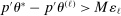 for all ℓ. Recall that along this subsequence,
  because
 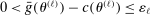 . We will construct
  s.t.
s.t. 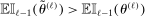 , contradicting the definition of
  .
.
By Assumption A.3,
 (A.17)
 . By the Cauchy–Schwarz inequality, for any
  ,
,
 (A.18)
 and noting that
  , we obtain
 (A.19)
 ,
,
 (A.20)

 s.t.
s.t.
 (A.21)
 , one can write
 (A.22)
 (A.23)
 . Lemma A.6 also yields

 (A.24)
 by (A.32) and
  by assumption. Hence,
  . This in turn implies
 (A.25)
The next lemma shows that, on  ,
,  and
and  are close to each other, where we recall that
  is the optimum value among the available feasible points (it belongs to
  ).
).
Lemma A.2.Suppose Assumptions A.1, A.2, and A.3 hold. Let  be a positive sequence such that
  and
and  . Then, there exists a constant
  such that
  for all L sufficiently large.
Proof.We show below  uniformly over
  for some decreasing sequence
  satisfying the assumptions of the lemma. The claim then follows by relabeling
  .
.
Suppose by contradiction that, for any  , there is a subsequence
  along which
  and
and  for all L sufficiently large. To simplify notation, we select a subsequence
  of
of  such that, for any
  ,
,  . This then induces a sequence such that
  for all ℓ, where each ℓ equals
  for some
  . Similarly to the proof of Lemma A.1, we omit the arguments of ℓ below and construct a sequence of points
  such that
  .
.
Arguing as in (A.17)–(A.20), one may find a sequence of points  such that
 (A.26)
 and for all ℓ sufficiently large. Furthermore, by Lemma A.1,
 (A.27)
 and for all ℓ sufficiently large. Arguing as in (A.23),
 (A.28)
 , and
, and  . Similarly, by Lemma A.6,
 (A.29)
 and one can find a subsequence
  so that
  for all ℓ sufficiently large.
Subtracting (A.28) from (A.29) yields

 s.t.
s.t.

 by (A.24), (A.32), and
  . Therefore, for all ℓ sufficiently large,

 for all ℓ sufficiently large, which implies
  for all ℓ sufficiently large. However, this contradicts the assumption that
  is the expected improvement maximizer. □
The next lemma shows that, on  ,
,  and
and  are close to each other.
Lemma A.3.Suppose Assumptions A.1, A.2, and A.3 hold. Let  be a positive sequence such that
  and
and  . Then, there exists a constant
  such that
  for all L sufficiently large.
Proof.Note that, for any  ,
,  , and
, and  ,
,  satisfies
  , hence
  , which in turn implies

 that ensures
  uniformly over
  for all L. Suppose by contradiction that, for any
  , there is a subsequence
  along which
  and
and  for all L sufficiently large. Again, we select a subsequence
  of
of  such that, for any
  ,
,  . This then induces a sequence
  of expected improvement maximizers such that
  for all ℓ, where each ℓ equals
  for some
  .
.Similarly to the proof of Lemma A.1, we omit the arguments of ℓ below and prove the claim by contradiction. Below, we assume that, for any  , there is a further subsequence along which
  for all ℓ sufficiently large.
Now let  with
with  specified below. By Assumption A.3, for all
  , it holds that

 and taking
  such that
  , it follows that
  for all ℓ sufficiently large.
Arguing as in (A.17)–(A.20), one may find a sequence of points  such that

 for all ℓ imply


 is the expected improvement maximizer. □
The next lemma shows that, on  ,
,  and
and  are close to each other.
Lemma A.4.Suppose Assumptions A.1, A.2, and A.3 hold. Let  for
for  . Let
. Let  . Then, there exists a constant
  such that
  for all L sufficiently large.
Proof.Let  be a sequence such that
  for all L. Since
  , there is
  such that
  and
and  is chosen by maximizing the expected improvement.
For later use, we note that, for any  , it can be shown that
  , which in turn implies that there exists a constant
  such that
 (A.30)
For  and
and  , let
, let  . Recall that
  is an optimal solution to (2.11). Then, for all L sufficiently large,

 being the maximizer of the expected improvement, (4) follows from Lemma A.5, (5) follows from (A.30) with
  , (6) follows from
  , (7) follows from Lemma A.5, (8) follows from
  being the expected improvement maximizer, (9) follows from Lemma A.5, and (10) follows from
  due to the definition of
  . This establishes the claim. □
For evaluation points  such that
  , the following lemma is an analog of Lemma 8 in Bull (2011), which links the expected improvement to the actual improvement achieved by a new evaluation point θ.
Lemma A.5.Suppose  is bounded and
  . Suppose the evaluation points
  are drawn by Algorithm A.1 and let Assumptions A.1 and A.2(ii) hold. For
  and
and  , let
, let  . Let
. Let  be a positive sequence such that
  and
and  . Let
. Let  . Then, for any sequence
  such that
  ,
,

 .
.
Proof of Lemma A.5.If  , then the posterior variance of
  is zero. Hence,
  , and the claim of the lemma holds.
Suppose  . We first show the upper bound. Let
  and
and  . By Lemma 6 in Bull (2011), we have
  . Starting from Lemma A.6(i), we can write
 (A.31)
 for any
  . Note that one may write

 , we will write
  . By the hypothesis that
  and Lemma 4 in Bull (2011), we have

 uniformly sampled points, and
  is associated with index
  . As shown in the proof of Theorem 5 in Bull (2011), this ensures that
 (A.32)
 . This, together with
  and the fact that
  is decreasing, yields
 (A.33)
 and where
  . Note that, by the triangle inequality,
 (A.34)
 (A.35)
 , where ϕ is the density of the standard normal distribution, and the inequality follows from
  . The second term on the right-hand side of (A.34) can be bounded as
 (A.36)
 is a point between
  and
and  . The claim of the lemma then follows from (A.31), (A.33)–(A.36), and
  being bounded because Θ is bounded.
Similarly, for the lower bound, we have
 (A.37)
 (A.38)
 . Arguing as in (A.37) and noting that
  is increasing, one has
 (A.39)
 and
and  . By the triangle inequality,
 (A.40)
 (A.41)
 (A.42)
 is a point between
  and
and  . The claim of the lemma then follows from (A.37)–(A.42), and
  being bounded because Θ is bounded. □
Lemma A.6.Suppose  is bounded and
  and let Assumptions A.1 and A.2(ii) hold. Let
  . For
. For  and
and  , let
, let  . Then, (i) for any
  and
and  ,
,

 and
and  such that
  ,
,
 (A.43)
 and
and  . By Lemma 6 in
  . Since
  is decreasing, we have


 and the fact that
  is decreasing. □
Appendix B: Applying the E-A-M Algorithm to Profiling
 denote the parameter space for
  . The (one-dimensional) profiling confidence region is

 is the critical value proposed in Bugni, Canay, and Shi (2017) and
  is any test statistic that they allowed for. The E-A-M algorithm can be used to compute the endpoints of this set so that the researcher may report an interval.
 (B.1)
(B.1) as a black box function and apply the E-A-M algorithm.35 We include the profiled statistic in the black box function because it involves a nonlinear optimization problem, which is also relatively expensive. The modified procedure is as follows.
- Initialization: Draw randomly (uniformly) over
 a set
a set  of initial evaluation points and evaluate
  for
for  . Initialize
  .
. - E-step: Evaluate
 and record the tentative optimal value

- A-step: (Approximation):
Approximate
 by a flexible auxiliary model. We again use the kriging approximation, which for a mean-zero Gaussian process
  indexed by τ and with constant variance
  specifies
where
specifies
where
 is a kernel with a scalar parameter
  . The parameters are estimated in the same way as before.
The (best linear) predictor of c and its derivative are then given by
where
 is a vector whose ℓth component is
  as given above with estimated parameters,
  , and
, and  is an L-by-L matrix whose
  entry is
  with estimated parameters. The amount of uncertainty left in
  is captured by the following variance:

- M-step: (Maximization): With probability
 , maximize the expected improvement function
  to obtain the next evaluation point, with
With probability
to obtain the next evaluation point, with
With probability
 , draw
  randomly from a uniform distribution over
  .
.
As before,  is reported as endpoint of
  upon convergence. In order for Theorem 3.2 to apply to this algorithm, the profiled statistic
  and the critical value
  need to be sufficiently smooth. We leave derivation of sufficient conditions for this to be the case to future research.
Appendix C: An Entry Game Model and Some Monte Carlo Simulations
We evaluate the statistical and numerical performance of calibrated projection and E-A-M in comparison with BCS-profiling in a Monte Carlo experiment run on a server with two Intel Xeon X5680 processors rated at 3.33 GHz with six cores each and with a memory capacity of 24 Gb rated at 1333 MHz. The experiment simulates a two-player entry game in the Monte Carlo exercise of BCS, using their code to implement their method.36
C.1 The General Entry Game Model
We consider a two-player entry game based on Ciliberto and Tamer (2009):
|
|
|
|
|
Y1 = 0 |
|
|
|
Y1 = 1 |
|
|


 ,
,  , and
, and  denote player ℓ's binary action, observed characteristics, and unobserved characteristics. The strategic interaction effects
  measure the impact of the opponent's entry into the market. We let
  . We generate
  as an i.i.d. random vector taking values in a finite set whose distribution
  is known. We let
  be independent of Z and such that
  and
and  ,
,  . We let
  . For a given set
  , we define
  . We choose
  so that the c.d.f. of u is continuous, differentiable, and has a bounded p.d.f. The outcome
  results from pure strategy Nash equilibrium play. For some value of Z and u, the model predicts monopoly outcomes
  and
and  as multiple equilibria. When this occurs, we select outcome
  by independent Bernoulli trials with parameter
  . This gives rise to the following restrictions:
 (C.1)
(C.1)C.2 A Comparison to BCS-Profiling
BCS specialized this model as follows. First,  ,
,  are independently uniformly distributed on
  and the researcher knows
  . Equality (C.1) disappears because
  is never an equilibrium. Next,
  , where
  are observed market-type indicators,
  for
for  , and
, and  .38 The parameter vector is
  with parameter space
  . This leaves four moment equalities and eight moment inequalities (so
  ); compare equation (5.1) in BCS. We set
  ,
,  ,
,  ,
,  , and
, and  . The implied true bounds on parameters are
  ,
,  ,
,  ,
,  , and
, and  .
.
The BCS-profiling confidence interval  inverts a test of
  over a grid for τ. We do not, in practice, exhaust the grid but search inward from the extreme points of Θ in directions ±p. At each τ that is visited, we use BCS code to compute a profiled test statistic and the corresponding critical value
  . The latter is a quantile of the minimum of two distinct bootstrap approximations, each of which solves a nonlinear program for each bootstrap draw. Computational cost quickly increases with grid resolution, bootstrap size, and the number of starting points used to solve the nonlinear programs.
Calibrated projection computes  by solving a series of linear programs for each bootstrap draw.39 It computes the extreme points of
  by solving the nonlinear program (2.4) twice, a task that is much accelerated by the E-A-M algorithm. Projection of Andrews and Soares (2010) operates very similarly but computes its critical value
  through bootstrap simulation without any optimization.
We align grid resolution in BCS-profiling with the E-A-M algorithm's convergence threshold of 0.005.40 We run all methods with  bootstrap draws, and calibrated and “uncalibrated” (i.e., based on Andrews and Soares (2010)) projection also with
  .41 Some other choices differ: BCS-profiling is implemented with their own choice to multi-start the nonlinear programs at three oracle starting points, that is, using knowledge of the true DGP; our implementation of both other methods multi-starts the nonlinear programs from 30 data-dependent random points (see Kaido et al. (2017) for details).
Table II displays results for  and for 300 Monte Carlo repetitions of all three methods. All confidence intervals are conservative, reflecting the effect of GMS. As expected, uncalibrated projection is most conservative, with coverage of essentially 1. Also, BCS-profiling is more conservative than calibrated projection. The most striking contrast is in computational effort. Here, uncalibrated projection is fastest—indeed, in contrast to received wisdom, this procedure is computationally somewhat easy. This is due to our use of the E-A-M algorithm and therefore part of this paper's contribution. Next, our implementation of calibrated projection beats BCS-profiling with gridding by a factor of about 70. This can be disentangled into the gain from using calibrated projection, with its advantage of bootstrapping linear programs, and the gain afforded by the E-A-M algorithm. It turns out that implementing BCS-profiling with the adapted E-A-M algorithm (see Appendix B) improves computation by a factor of about 4; switching to calibrated projection leads to a further improvement by a factor of about 17. Finally, Table III extends the analysis to all components of θ and to 1000 Monte Carlo repetitions. We were unable to compute this for BCS-profiling.
 ,
,  ,
,  ,
,  ,
,  a
a|
Median CI |
|||||
|---|---|---|---|---|---|
|
|
|
|
|||
|
Implementation |
|
Grid |
E-A-M |
E-A-M |
E-A-M |
|
|
0.95 |
[0.330,0.495] |
[0.331,0.495] |
[0.336,0.482] |
[0.290,0.558] |
|
0.90 |
[0.340,0.485] |
[0.340,0.485] |
[0.343,0.474] |
[0.298,0.543] |
|
|
0.85 |
[0.345,0.475] |
[0.346,0.479] |
[0.348,0.466] |
[0.303,0.537] |
|
|
|
0.95 |
[0.515,0.655] |
[0.514,0.655] |
[0.519,0.650] |
[0.461,0.682] |
|
0.90 |
[0.525,0.647] |
[0.525,0.648] |
[0.531,0.643] |
[0.473,0.675] |
|
|
0.85 |
[0.530,0.640] |
[0.531,0.642] |
[0.539,0.639] |
[0.481,0.671] |
|


|
Coverage |
|||||||||
|---|---|---|---|---|---|---|---|---|---|
|
|
|
|
|||||||
|
Grid |
E-A-M |
E-A-M |
E-A-M |
||||||
|
Implementation |
|
Lower |
Upper |
Lower |
Upper |
Lower |
Upper |
Lower |
Upper |
|
|
0.95 |
0.997 |
0.990 |
1.000 |
0.993 |
0.993 |
0.977 |
1.000 |
1.000 |
|
0.90 |
0.990 |
0.980 |
0.993 |
0.977 |
0.987 |
0.960 |
1.000 |
1.000 |
|
|
0.85 |
0.970 |
0.970 |
0.973 |
0.960 |
0.957 |
0.930 |
1.000 |
1.000 |
|
|
|
0.95 |
0.987 |
0.993 |
0.990 |
0.993 |
0.973 |
0.987 |
1.000 |
1.000 |
|
0.90 |
0.977 |
0.973 |
0.980 |
0.977 |
0.940 |
0.953 |
1.000 |
1.000 |
|
|
0.85 |
0.967 |
0.957 |
0.963 |
0.960 |
0.943 |
0.927 |
1.000 |
1.000 |
|


|
Average Time |
|||||
|---|---|---|---|---|---|
|
|
|
|
|||
|
Implementation |
|
Grid |
E-A-M |
E-A-M |
E-A-M |
|
|
0.95 |
1858.42 |
425.49 |
26.40 |
18.22 |
|
0.90 |
1873.23 |
424.11 |
25.71 |
18.55 |
|
|
0.85 |
1907.84 |
444.45 |
25.67 |
18.18 |
|
|
|
0.95 |
1753.54 |
461.30 |
26.61 |
22.49 |
|
0.90 |
1782.91 |
472.55 |
25.79 |
21.38 |
|
|
0.85 |
1809.65 |
458.58 |
25.00 |
21.00 |
|


- a
(1) Projections of
 are:
are:  ,
,  ,
,  ,
,  ,
,  . (2) “Upper” coverage is for
  , and similarly for “Lower”. (3) “Average time” is computation time in seconds averaged over MC replications. (4)
  results from BCS-profiling,
  is calibrated projection, and
  is uncalibrated projection. (5) “Implementation” refers to the method used to compute the extreme points of the confidence interval.
 ,
,  ,
,  ,
,  ,
,  a
a|
Median CI |
|
|
Average Time |
||||||
|---|---|---|---|---|---|---|---|---|---|
|
|
|
|
Lower |
Upper |
Lower |
Upper |
|
|
|
|
|
0.95 |
[0.333,0.478] |
[0.288,0.555] |
0.988 |
0.982 |
1 |
1 |
42.41 |
22.23 |
|
0.90 |
[0.341,0.470] |
[0.296,0.542] |
0.976 |
0.957 |
1 |
1 |
41.56 |
22.11 |
|
|
0.85 |
[0.346,0.464] |
[0.302,0.534] |
0.957 |
0.937 |
1 |
1 |
40.47 |
19.79 |
|
|
|
0.95 |
[0.525,0.653] |
[0.466,0.683] |
0.969 |
0.983 |
1 |
1 |
42.11 |
24.39 |
|
0.90 |
[0.538,0.646] |
[0.478,0.677] |
0.947 |
0.960 |
1 |
1 |
40.15 |
28.13 |
|
|
0.85 |
[0.545,0.642] |
[0.485,0.672] |
0.925 |
0.941 |
1 |
1 |
41.38 |
26.44 |
|
|
|
0.95 |
[0.054,0.142] |
[0.020,0.180] |
0.956 |
0.958 |
1 |
1 |
40.31 |
22.53 |
|
0.90 |
[0.060,0.136] |
[0.028,0.172] |
0.911 |
0.911 |
1 |
1 |
36.80 |
24.15 |
|
|
0.85 |
[0.064,0.132] |
[0.032,0.167] |
0.861 |
0.860 |
0.999 |
0.999 |
39.10 |
21.81 |
|
|
|
0.95 |
[0.156,0.245] |
[0.121,0.281] |
0.952 |
0.952 |
1 |
1 |
39.23 |
24.66 |
|
0.90 |
[0.162,0.238] |
[0.128,0.273] |
0.914 |
0.910 |
0.998 |
0.998 |
41.53 |
21.66 |
|
|
0.85 |
[0.165,0.234] |
[0.133,0.268] |
0.876 |
0.872 |
0.996 |
0.996 |
39.44 |
22.83 |
|
|
|
0.95 |
[0.257,0.344] |
[0.222,0.379] |
0.946 |
0.946 |
1 |
1 |
41.45 |
22.91 |
|
0.90 |
[0.263,0.338] |
[0.230,0.371] |
0.910 |
0.909 |
0.997 |
0.999 |
42.09 |
22.83 |
|
|
0.85 |
[0.267,0.334] |
[0.235,0.366] |
0.882 |
0.870 |
0.994 |
0.993 |
42.19 |
23.69 |
|
 Coverage
 Coverage


- a Same DGP and conventions as in Table II.
In sum, the Monte Carlo experiment on the same DGP used in BCS yields three interesting findings: (i) the E-A-M algorithm accelerates projection of the Andrews and Soares (2010) confidence region to the point that this method becomes reasonably cheap; (ii) it also substantially accelerates computation of profiling intervals, and (iii) for this DGP, calibrated projection combined with the E-A-M algorithm has the most accurate size control while also being computationally attractive.