The coupling torque signal contains essential information about the operating condition of the motor-follower mechanical system. Artificial Intelligence methods have been effective in diagnosing coupling faults. However, due to internal and external excitations caused by the operating environment and neighboring components, existing coupling fault diagnosis models often struggle with poor feature extraction, low recognition accuracy, and weak generalization performance. To overcome these limitations, a multihead self-attention mechanism-enhanced empirical mode decomposition (EEMD)–convolutional neural network (CNN)–bidirectional long short-term memory (BiLSTM) model is proposed. Empirical mode decomposition (EMD) is first applied to extract spatial features from the data. Next, the multihead self-attention mechanism captures essential internal characteristics. CNN is then used for further spatial feature extraction, and BiLSTM is employed to extract temporal features, enabling effective spatiotemporal feature fusion. Torque and vibration signals of three typical coupling faults—loosening, rough contact, and misalignment—are collected using a motor-coupling-paper handling mechanism testbed and compared with traditional models, including long short-term memory (LSTM), CNN, and Random Forest. The proposed method shows an average F1-Score improvement of 31.43%, 40.07%, and 31.71%, respectively, indicating superior noise robustness and better generalization. Furthermore, the dimensionality reduction results of each network layer are visualized using the T-stochastic neighbor embedding (T-SNE) method, which reveals clear feature patterns and confirms the model’s reliability and effectiveness.

1. Introduction

As a vital transmission component in mechanical systems, the coupling plays a key role in connecting and transmitting torque, enabling the active rotary shaft in different mechanisms to drive the passive rotary shaft for synchronized rotary motion. Among various types, the plum-blossom flexible coupling has been widely used in high-torque and high-speed operations due to its compact design, high transmission capacity, and other advantages. It has been applied in fields such as drive systems, aviation systems, and printing systems, providing flexibility and high efficiency for modern engineering [1, 2]. In a printing system, the paper feeder feeds paper sheets from the paper stack into the printing device one at a time. During this process, power is transmitted through a plum-blossom flexible coupling that connects the motor to the bearings of the delivery mechanism, ensuring the continuous operation of the system.

Plum-blossom flexible couplings in paper delivery mechanisms are subject to high-speed rotation and complex loads, making them vulnerable to failure modes such as coupling misalignment [3], loosening of expansion bolts [4], and rough contact [5]. These issues threaten not only the coupling’s performance but also the stability of the entire system. Fault diagnosis is crucial to ensure system reliability [6]. For example, in the study of misalignment faults, Xuan et al. [7] observed that vibration signals caused by misalignment in plum-blossom flexible couplings on ship hydraulic pumps did not show significant line spectrum frequencies at motor rotational frequencies. Similarly, Dos [8], Hujare and Karnik [9], Chandra and Sekhar [10], and Guo et al. [11] emphasized that prolonged misalignment can impair system performance and cause severe failures, with the vibration spectrum significantly changing over time. On the topic of bolt loosening, Jiang et al. [12] focused on the dynamic effects of bolt loosening and microsliding on threaded and curved surfaces. Zhang et al. [13] investigated loosening in coupling connections used in cranes, highlighting the critical importance of connection reliability for safe operation. In addition, Li [5] discovered that coupling vibration signals exhibit nonlinearity in the early stages of faults, making accurate fault modeling and identification challenging.

The long short-term memory (LSTM) neural network, as an advanced variant of the recurrent neural network (RNN), was capable of handling long sequences while mitigating issues such as gradient vanishing and gradient explosion [14–16]. Compared with other commonly used deep learning models, such as GRU [17] and XGBoost [18], LSTM offers several advantages in processing faulty time-series data. It could manage variable-length sequences and was well suited for fault diagnosis tasks across different devices and systems [19, 20]. However, as research on LSTM advanced, scholars identified several limitations, including insufficient forgetting capability and the need for larger training datasets [21]. To address these limitations, studies introduced the bidirectional long short-term memory (BiLSTM) neural network, which improved fault diagnosis performance by integrating forward and backward sequence information, thereby enhancing the model’s ability to capture long-term dependencies [22–24]. For instance, Song et al. [25] applied a convolutional neural network (CNN)–BiLSTM network as a pretrained model with limited training data for bearing fault diagnosis under varying operating conditions, achieving better detection accuracy. Compared with a single CNN model and LSTM model, the recognition accuracy and recall increased by 1.36% and 0.705%, while the F1-Score improved by 1.369% and 0.72%, respectively. In this study, to enhance the classification and recognition accuracy of coupling faults by mining data features, a feature extraction module was developed, with the BiLSTM neural network selected as the core training model.

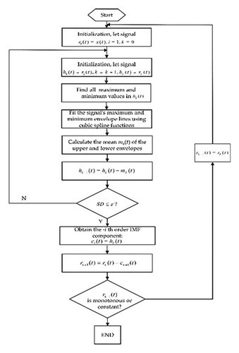
Effective decomposition of data signals can enhance model accuracy and improve feature representation. Liu [26] and Li et al. [6] used ensemble empirical modal decomposition (EEMD) to break down fault signals from reservoir gate opener couplings and wind turbine couplings, improving the model’s ability to diagnose weak fault signals. Jiao [27] combined the empirical mode decomposition (EMD) method with LSTM to enhance temporal feature extraction, resulting in higher accuracy than BP, RNN, and LSTM models without EMD processing. While variational mode decomposition (VMD) could provide more precise signal decomposition [28], it requires predefining modes and adjusting penalty parameters [29], which adds complexity. In contrast, EMD is adaptive [30], requiring no preset modes, making it more suitable for complex and uncertain signal characteristics. EMD is also effective for handling nonstationary and nonlinear signals commonly seen in mechanical systems, offering a reliable foundation for fault diagnosis in complex environments. Thus, EMD was chosen for signal decomposition in this study due to its balance of accuracy and practical deployment.

CNN is effective in capturing image features and patterns [31, 32] and also improves the accuracy of temporal models. By extracting spatial information through convolutional operations, CNN enhances the combined model, allowing it to perform both temporal and spatial feature extraction [33]. Fu et al. [34] used CNN to extract spatial features from time–frequency data obtained from BiLSTM. Using a parallel neural network, Fu’s approach outperformed traditional machine learning and deep learning methods in fault identification using datasets from Case Western Reserve University and Jiangnan University. Similarly, Kavianpour et al. [35] applied a CNN–BiLSTM model for earthquake prediction, effectively extracting spatial information with CNN.

Attention mechanisms are often integrated into deep learning models to enhance focus on relevant features during extraction and are widely applied in image processing [36] and other data-driven fields [37]. Xie et al. [38] used Attention–BidiRNN and Attention–BidiLSTM models, achieving accuracy improvements of 9.05% and 4.7%, respectively. Dong et al. [39] proposed a position encoding-based attention mechanism for predicting the future motion of ships in real sea environments.

This study first applies EMD to adaptively decompose various types of fault signals, extracting high-frequency, low-frequency, and trend information to maximize data feature representation of the target. Next, a multihead self-attention mechanism is introduced, enabling the model to automatically focus on targets with varying positional and angular features. Subsequently, CNN with a sliding convolution kernel is employed to extract spatial information from the data. Finally, the BiLSTM neural network is integrated to capture temporal information, ensuring precise fault identification.

2. Data Resource

2.1. Data Preprocessing

The quality of data collected during experiments directly affects the model’s performance and reliability. Several preprocessing measures were applied to minimize data errors and enhance the model’s robustness, ensuring effective feature extraction and strong generalization.

During the experiments, signal acquisition in industrial environments is often accompanied by noise and outliers, which can negatively affect feature extraction and model training. Therefore, noise inspection and processing of the collected torque signals are necessary to ensure effective model training and robustness. Figure 1 illustrates the frequency domain diagrams obtained through the Fourier transform for normal, loosening, rough contact, and misalignment conditions, with a time sampling interval of 0.005. From the figure, it can be observed that the main frequency components are concentrated in the low-frequency range, while the high-frequency range contains a certain level of noise. This high-frequency noise primarily originates from external environmental interference and sensor precision limitations.

Details are in the caption following the image — **Figure 1**
Open in figure viewer PowerPoint

The frequency domain diagrams of different faults. (a) Normal. (b) Loosening. (c) Rough contact. (d) Misalignment.

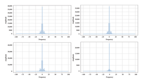
An outlier filtering method was adopted to reduce the impact of noise on model training. Abnormal data were filtered out by setting reasonable upper and lower threshold limits, while samples with fluctuation characteristics were retained to verify the model’s robustness. Outliers, identified as samples with fluctuation amplitudes significantly exceeding the normal range and inconsistent with actual operating conditions, were removed. In contrast, samples with slight fluctuations were kept to improve the model’s adaptability to noise.

2.2. Data Details

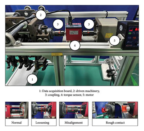
A motor-coupling-paper delivery mechanism test bed was constructed in this study to collect fault signal data. Torque was transmitted from the motor to the paper delivery mechanism via a flexible coupling, driving its operation. The motor had a power rating of 0.75 kW and a speed range of 0–1500 rpm. Data acquisition was carried out using a DYN-200 dynamic torque sensor with a precision of 0.1% and a rated capacity of ±10,000 Nm. The setup included two GFS-40X55 elastic couplings. A variable frequency drive adjusted the motor speed to simulate different operating conditions, and torque signals were collected under normal conditions and three fault conditions: loosening, misalignment, and rough contact. The loosening fault was simulated by reducing the clamping force of the coupling bolts, the misalignment fault by offsetting the axes of the drive and load shafts and the rough contact fault by slightly wearing down the elastic elements inside the coupling to induce abnormal friction. Detailed descriptions of the faults and their parameters are provided in Table 1 to ensure the controllability and reproducibility of experimental conditions. The experimental platform setup and specific fault details are illustrated in Figure 2.

Table 1. Fault specific settings.

Fault type	Fault description	Fault parameters	Sampling frequency (Hz)	Motor speed (rpm)
Normal	Coupling installed properly without any faults	Coupling assembled following standard procedures with axial alignment deviation controlled within 0.05 mm	100	595
Loosening	Insufficient clamping force causing loose connection	Fastening bolts loosened by 1/2 turn, with a looseness gap of about 2 mm	100	595
Misalignment	Axial misalignment on both sides of the coupling	Axial offset of 2 mm between the drive and load shafts, with an offset angle of 1.5°	100	595
Rough contact	Wear on the elastic elements during coupling operation	Wear depth of elastic elements inside the coupling is 0.5 mm	100	595

The sampling frequency of measured data is 100 Hz. Rotational speed is 595 revolutions per minute (rpm). The data of normal and faulty conditions of the coupling measured are shown in Figure 3.

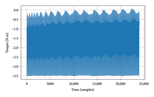
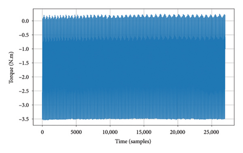
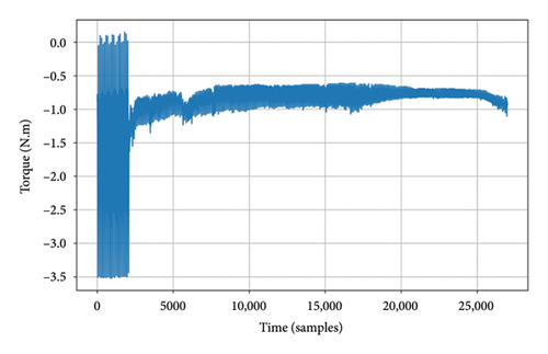
As shown in Figure 3, the torque signals exhibit distinct characteristics under normal and different fault conditions. Under normal conditions, the torque signals display approximately periodic fluctuations, with consistent intervals between peaks and valleys and no noticeable irregularities. In the case of loosening faults, the torque signal loses its periodicity, and the intervals between peaks and valleys vary significantly, indicating unstable torque transmission caused by the loosening of the coupling. For rough contact faults, the torque signal shows a significant reduction in the intervals between peaks and valleys, resulting in a shorter fluctuation period. This reflects an increase in friction resistance within the coupling. In misalignment faults, the torque signal reveals a sudden decrease in torque amplitude during the measurement process, along with abnormal fluctuations. This indicates an unbalanced load between the rotating components due to shaft misalignment, leading to additional friction and vibration during operation.

3. Methods

3.1. Data Standardization

To enhance the robustness of the model to outliers, the data are normalized to standardize the features and speed up model training.

\begin{matrix} X^{*} = \frac{X - \min (X)}{\max (X) - \min (X)}, \end{matrix}

()

where X^∗ denotes the standardized data result. X represents the original data. The min(X) signifies the minimum value within the column. The max(X) signifies the maximum value within the column.

3.2. EMD

EMD plays a crucial role in fault diagnosis by effectively decomposing complex, nonstationary, and nonlinear signals into intrinsic mode functions (IMFs), thus extracting important features from fault signals [40]. The decomposition of the signal allows the fault characteristics to be more clearly presented, especially when the fault features are weak or masked by noise. By breaking the signal into multiple components, EMD can effectively enhance the feature representation of different types of faults. In addition, EMD is adaptive and does not require preset parameters, making it highly suitable for practical fault diagnosis applications, particularly when the signal behavior varies significantly.

\begin{matrix} x (t) = Im f_{1} (t) + Im f_{2} (t) + \dots + Im f_{N} (t) + r_{N} (t), \end{matrix}

()

where x(t) is the original functions. Imf₁(t), Imf₂(t), and Imf_N(t) represent the split N eigenmode functions. r_N(t) represents the residuals. The flowchart of the algorithm is obtained as shown in Figure 4.

3.3. Fault Diagnosis Classification Model

3.3.1. BiLSTM Neural Network Model

LSTM handled long-term dependencies in sequential data, maintained long-term memory increased the stability of backpropagation, and reduced the challenges of gradient disappearance and gradient explosion during training [41]. Its structure is shown in Figure 5.

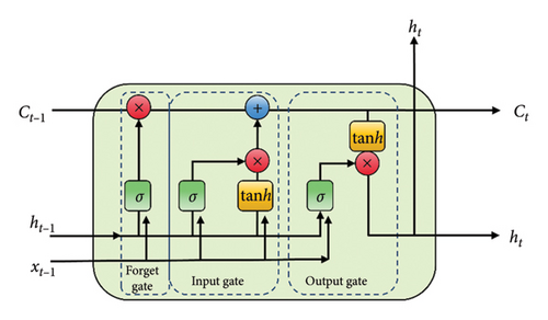
Its cell structure mainly consists of three gating mechanisms and one cell state. The gating mechanisms are input gate i_t, output gate O_t, and forget gate f_t. At time t − 1, the LSTM cell receives inputs C_t−1, h_t−1, and x_t−1, while at time, it outputs C_t, h_t, and x_t.

The forgetting gate is utilized to regulate the extent of memory loss in a cell state, determining whether the information in the preceding cell state C_t−1 should be preserved or discarded. The value of the forgetting gate output f_t is governed by the sigmoid function.

\begin{matrix} f_{t} = σ (W_{f} \cdot [h_{t - 1}, x_{t}] + b_{f}), \end{matrix}

()

where the input of the current instant is represented by x_t, the hidden state of the previous moment by h_t−1, the bias vector by b_f, and the weight matrix of forgetting gate by W_f.

Input gates are used to decide what x_t information needs to be added to the cell state in the current moment. The output of the input gates i_t is determined by a sigmoid function.

\begin{matrix} i_{t} = σ (W_{i} \cdot [h_{t - 1}, x_{t}] + b_{i}), \\ {\tilde{C}}_{t} = \tanh (W_{C} \cdot [h_{t - 1}, x_{t}] + b_{C}), \end{matrix}

()

where the updated candidate cell state is represented by

{\tilde{C}}_{t}

. The bias vector is represented by b_i. The weight matrix is represented by W_i and W_c.

The process of updating the cell state is a merge update through a gating mechanism. The following formula determines the updated cell state.

\begin{matrix} C_{t} = f_{t}^{*} C_{t - 1} + i_{t}^{*} {\tilde{C}}_{t}, \end{matrix}

()

where the updated cell state is denoted by

{\tilde{C}}_{t}

whereas the old cell state is represented by C_t−1.

The sigmoid function determines the output O_t of the output gate, which is used to determine how much information in the hidden state is now needed to be sent on to the next output layer.

\begin{matrix} O_{t} = σ (W_{o} [h_{t - 1}, x_{t}] + b_{o}), \\ h_{t} = O_{t}^{*} \tanh (C_{t}), \end{matrix}

()

where the current cell state is represented by C_t. The ultimate output is represented by h_t. The bias vector is represented by b_∘. The weight matrix of the output gate is represented by W_o.

The BiLSTM neural network extends the capabilities of the LSTM by processing sequential data bidirectionally, integrating both forward and backward information. This allows for more effective capture of long-term dependencies and local features within the data, enhancing the accuracy of fault differentiation [42]. The structure of the BiLSTM neural network model is shown in Figure 6.

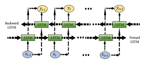
Here, the LSTM unit receives x_t−1 as input information at time t − 1 and likewise receives x_t and x_t+1 as input information at time t and t + 1, respectively. The final output at time t − 1 is denoted by y_t−1. Similarly, y_t and y_t+1 are the final output at the moment of t and t + 1, respectively. For each input, a forward and a backward LSTM unit are used for feature extraction and processing of the information.

The computational process of the BiLSTM network model is shown in the following.

\begin{matrix} {\overset{⟶}{h}}_{t} = f (\overset{⟶}{w} x_{t} + \overset{⟶}{v} {\overset{⟶}{h}}_{t - 1} + \overset{⟶}{b}), \end{matrix}

()

\begin{matrix} {\overset{\leftarrow}{h}}_{t} = f (\overset{\leftarrow}{w} x_{t} + \overset{\leftarrow}{v} {\overset{\leftarrow}{h}}_{t + 1} + \overset{\leftarrow}{b}), \end{matrix}

()

where equation (7) is the forward LSTM hidden state vector computation expression, where the forward LSTM hidden state at time step t and at time t − 1 is denoted by the

{\overset{⟶}{h}}_{t}

and

{\overset{⟶}{h}}_{t - 1}

. The input weights at times t and t − 1 are represented by the

\overset{⟶}{w}

and

\overset{⟶}{v}

\overset{⟶}{b}

denotes the LSTM layer bias vector. f(·) denotes the activation function. Similarly, the equation for backward LSTM hidden state computation is given by equation (8).

\begin{matrix} y_{t} = g (U [{\overset{⟶}{h}}_{t}; {\overset{⟵}{h}}_{t}] + c), \end{matrix}

()

where y_t represents the final output at time t.

[{\overset{⟶}{h}}_{t}; {\overset{⟵}{h}}_{t}]

is the bidirectional hidden state formed by merging and superimposing the forward and backward hidden states.

3.3.2. CNN

CNN’s main method was to use convolutional and pooling processes to pull out localized data characteristics. This facilitated the process of hierarchical feature abstraction and extraction by leveraging a network structure with several layers [43]. The ReLU activation function is introduced to enhance the nonlinear function feature extraction capability of the network and better approximate the complex patterns in the faulty time-series data. The expression of its activation function is given in the following equation.

\begin{matrix} f (x) = \max (0, x) . \end{matrix}

()

3.3.3. Multihead Self Attention Mechanism

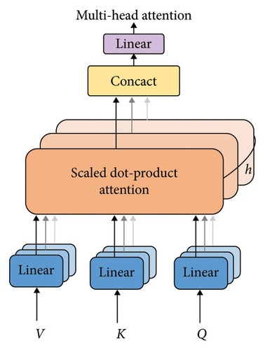
The attention mechanism dynamically adjusts the weights of elements in the input sequence [44], enabling the model to focus on the most critical information when processing sequential data. In the proposed EMD–CNN–BiLSTM model, the multihead self-attention mechanism is employed to extract fault features across different time scales and frequency ranges, thereby enhancing the model’s ability to understand complex signals. Compared with single-head attention, the multihead self-attention mechanism captures diverse features through multiple parallel “heads,” ensuring that the model can identify global trends while extracting local details [45]. For instance, in fault diagnosis, misalignment faults may only exhibit prominent characteristics within specific frequency ranges or time windows. The multihead self-attention mechanism can simultaneously focus on features at different scales, improving the detection capability for various types of faults. By incorporating the multihead self-attention mechanism into the BiLSTM network, the model can more accurately learn the dynamic characteristics of signals over time, reduce the risk of overfitting, and enhance generalization. Figure 7 illustrates the workflow of the multihead self-attention mechanism.

As shown in Figure 7, the multihead self-attention mechanism begins by applying linear transformations to the input sequence to generate the Query (Q), Key (K), and Value (V) matrices. These matrices are then divided into multiple lower-dimensional subspaces, with each subspace corresponding to a “head,” enabling different heads to focus on learning distinct features of the sequence. Next, for each head, the dot product of Q and K is computed to obtain relevance weights, which are normalized using the softmax function. The normalized weights are then used to perform a weighted sum on V, producing the attention output for each head. Finally, the outputs from all heads are concatenated and passed through a linear transformation to produce the final multihead self-attention result. The core formula is as follows.

\begin{matrix} MultiHead (Q, K, V) = Concat (hea d_{1}, hea d_{2}, \dots, hea d_{n}) W^{o}, \end{matrix}

()

where Concat(·) is to vertically splice the matrix.

W^{o} \in R^{h d_{ν} \times d_{model}}

is the weight matrix, and head_i is as follows.

\begin{matrix} hea d_{i} = Attention (Q W_{i}^{Q}, K W_{i}^{K}, V W_{i}^{V}), \end{matrix}

()

where

W_{i}^{K} \in R^{d_{model \times d_{k}}}

W_{i}^{V} \in R^{d_{model \times d_{v}}}

, and

W_{i}^{Q} \in R^{d_{model \times d_{q}}}

are weight matrices.

3.3.4. Optimized EMD–CNN–BiLSTM Model With Multihead Self-Attention Mechanism

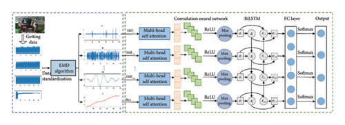
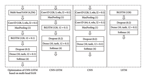
The EMD–CNN–LSTM fault diagnosis model is optimized based on a multihead self-attention mechanism consists of a data decomposition module (EMD), complex mechanism extraction module (multihead self-attention mechanism), fault feature extraction module (CNN), temporal dependency extraction module (LSTM neural network), overfitting prevention module (L2 regular term, gradient trimming technique), multiclassification output (Softmax function), and other modules.

The overall process is as follows. First, the raw torque data are decomposed into multiple IMFs using EMD, isolating key features while reducing irrelevant noise to provide cleaner and more information-rich input for subsequent processing. Next, the data are fed into the multihead self-attention mechanism, where multiple attention heads capture patterns across different frequencies or time scales, enabling the extraction of both fine-grained local features and global trends. Afterward, the data pass through a series of 1D convolutional layers and max-pooling layers. The convolutional layers, by scanning with kernels, detect patterns such as peaks, trends, and abrupt changes, while the max-pooling layers reduce data dimensionality and eliminate redundant information, thereby improving the model’s generalization ability. Following local feature extraction, the data are input into the LSTM network. As a sequential model, LSTM is well-suited for learning dependencies in time-series data. By employing a bidirectional structure, it considers both past and future context, allowing for more accurate capture of dynamic changes. To prevent overfitting, the model incorporates L2 regularization and Dropout. L2 regularization enhances generalization by penalizing large weights, while Dropout randomly deactivates a fraction of neurons, increasing model robustness. Finally, the extracted features are passed to the Softmax layer, which converts them into a probability distribution over the fault categories. The category with the highest probability is selected as the prediction result. For example, if the input data correspond to a “misalignment” fault, the Softmax layer assigns a high probability to that category and the model outputs “misalignment” as the predicted fault type. Figure 8 shows the overall structure of the model.

3.4. Performance Index

Accuracy, recall, and F1-Score are used to assess the model’s classification performance, as defined in equations [13]. Accuracy shows the proportion of correct predictions, with a higher value indicating better performance. Recall measures the correct identification of positive samples, while the F1-Score balances precision and recall, with a higher value reflecting better overall performance.

\begin{matrix} Accuracy = \frac{T P + T N}{T P + T N + F P + F N}, \\ Recall = \frac{T P}{T P + F N}, \\ F 1 = \frac{2 T P}{2 T P + F P + F N}, \end{matrix}

()

where TP is true positive, which can predict positive cases as positive cases. TN is true negative, which predicts negative cases as negative cases. FP is false positive, which predicts negative cases as positive cases. FN is false negative, which predicts positive cases as negative cases. Because the study considered a multicategorical problem, the subsequent evaluation of indicators was assessed by first calculating the indicator values for each category and then calculating the mean values.

4. Fault Detection Results Analysis

The multihead self-attention mechanism-optimized EMD–CNN–BiLSTM model is used to train, validate, and test the coupling operation data to judge the reasonableness of the model establishment.

4.1. Enhanced Representation of Data Features

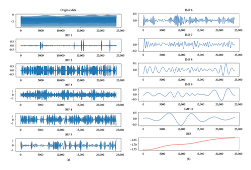
The original torque data is highly nonlinear, volatile, and unstable, with unclear features, making it difficult for model construction. To overcome this, EMD is used to decompose the data, separating simple fluctuations from complex signals and extracting features at different time scales. This enhances the data’s expressiveness, increases input diversity, and improves prediction accuracy.

Using normal data as an example, the data were decomposed into 10 IMFs and 1 residual (Res) group. IMF1 represents high-frequency noise, IMF2–IMF5 capture mid-frequency oscillations, reflecting the data’s dynamics at a medium time scale, and IMF6–IMF9 highlight low-frequency oscillations, showing slow trends and basic data features. IMF10 represents the overall trend, while the Res variable captures nonperiodic residual features. The decomposition shows that the data stabilize as it transitions from fluctuations, revealing consistent change patterns. This enables more effective extraction of features for improving modeling accuracy, such as with LSTM neural networks, as shown in Figure 9.

4.2. Validation of Fault Detection Model Effectiveness

4.2.1. Model Parameters

Experiments choose the Tensorflow2.10.0 Version of the deep learning environment, selected Keras2.10.0 to build the network, and the model constructor for sequential. The network is iteratively trained to get the optimal hyperparameters. According to the experiments, it can be seen that the highest precision is when the parameters are set as shown in the table, where because the network structure is more complex, so we select the regular term L2 with the Dropout method to prevent network overfitting. The parameters of the model are shown in Table 2.

Table 2. Model parameter settings.

Network infrastructure	Parameterization
Multihead self-attention mechanism	Attention head = 4 Attention head key = 256
Convolutional layer	Convolutional kernel = 128 Convolution kernel size = 3 activation = ReLU Padding = same kernel_regularizer = l2 (0.1)
Maximum pooling layer	Pool_size = 1
BiLSTM layer	Neurons = 128
Dropout	0.2
Full connectivity layer	Neurons = 32 activation = tanh Kernel_regularizer = l2 (0.1)
Final fully connected layer	Activation = Softmax

As shown in Table 2, the model parameters are set to optimize performance. Four attention heads and 256-dimensional keys were used to balance feature extraction and computational efficiency. A lower number of heads limits feature diversity, while a higher key dimension increases complexity [46]. The convolutional layer has 128 kernels with a kernel size of 3, effective for capturing local patterns and maintaining generalization, as shown in recent studies [47]. The ReLU activation function introduces nonlinearity, speeds up convergence, and mitigates the vanishing gradient problem [48]. L2 regularization is applied with a factor of 0.1 to prevent overfitting and maintain generalization [49]. Max-pooling layers reduce dimensionality while preserving key features, with a pool size of 1 to minimize complexity for small datasets [50]. BiLSTM with 128 neurons captures temporal dependencies, and the bidirectional structure improves dynamic signal modeling. To prevent overfitting, a 0.2 dropout rate is used, which is effective for small to medium datasets without slowing convergence [51].

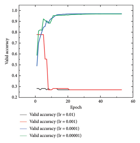
For network training, 70% of the data were used for training, 10% for validation, and 20% for testing. The Adam optimizer was employed for LSTM training, and the optimal batch size of 32 was selected based on experimental comparisons (Table 3), which achieved the best performance across all metrics with a 96.98% accuracy and an average training time of 40 s per epoch. Smaller batch sizes (16) increased training time and reduced performance, while larger batch sizes (64 and 128) led to poorer results, with an F1-Score of only 66.62% for 64, showing that larger batches hindered feature extraction and generalization. The batch size of 32 struck the best balance between performance and efficiency. A dynamic learning rate strategy, starting at 0.0001 and decreasing by a factor of 0.1 every 10 epochs, was used to improve convergence and avoid local minima. Experimental results (Figure 10) showed that a starting learning rate of 0.0001 yielded the best validation accuracy, while higher rates (0.01 and 0.001) caused instability, and a lower rate (0.00001) slowed convergence. To prevent overfitting, early stopping was applied based on validation loss.

Table 3. Comparison of model performance with different batch sizes.

Batch size	Accuracy (%)	Recall (%)	F1-Score (%)	Training time (s/epoch)
16	82.93	82.41	82.73	54
32	96.98	96.98	96.98	40
64	78.06	75.00	66.62	31
128	85.61	83.53	83.51	35

Note: The bold values show that the model performs best with a Batch size of 32.

4.2.2. Model Test Results

In order to confirm the validity of the suggested model, the test outcomes are contrasted and validated using the identical conventional CNN model, LSTM model with the same number of neurons, and EMD-optimized CNN–LSTM model. The parameters of each junction are shown in Figure 11.

The results from multiple experiments show that the model begins to converge after 54 iterations, with early stopping observed. The iteration accuracy of CNN, LSTM, EMD–CNN–LSTM, and the EMD–CNN–LSTM model optimized with a multihead self-attention mechanism on the validation set is visualized to assess the training effectiveness, as shown in Figure 12.

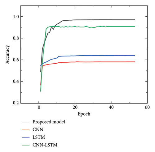
Figure 12 shows that the multihead self-attention mechanism-optimized EMD–CNN–LSTM model proposed has the highest accuracy in the valid set, which has the ability to extract feature information from torque and other data more effectively and provide a feasible, high-precision solution for fault diagnosis. To further validate the effectiveness of the model, the proposed model was tested three times using the test set to prevent the high accuracy on the validation set from being a result of overfitting. In addition, based on current research findings, models such as Random Forest [52] have demonstrated significant advantages in fault detection, so they were included for comparison. The results of three tests on the test set, using the best weights obtained after early stopping for each model, are presented in Table 4 and Figure 13.

Table 4. Test set detection performances.

Metrics		Methods
Metrics		Final model	CNN	LSTM	EMD–CNN–LSTM	Random Forest
1	Accuracy	0.9698	0.5894	0.6454	0.9088	0.6445
	Recall	0.9698	0.5894	0.6454	0.9088	0.6445
	F1-Score	0.9698	0.5536	0.6390	0.9084	0.6432

2	Accuracy	0.9667	0.5725	0.6978	0.9089	0.6463
	Recall	0.9663	0.5574	0.6955	0.9007	0.6463
	F1-Score	0.9637	0.5594	0.6195	0.9003	0.6465

3	Accuracy	0.9596	0.5715	0.6856	0.9044	0.6455
	Recall	0.9536	0.5715	0.6856	0.9117	0.6455
	F1-Score	0.9535	0.5718	0.6856	0.8993	0.6458

Average	Accuracy	0.9654	0.5778	0.6763	0.9074	0.6454
	Recall	0.9632	0.5728	0.6755	0.9071	0.6454
	F1-Score	0.9623	0.5616	0.6480	0.9027	0.6452

Note: The bold values reflect the fact that the final model has the best classification results.

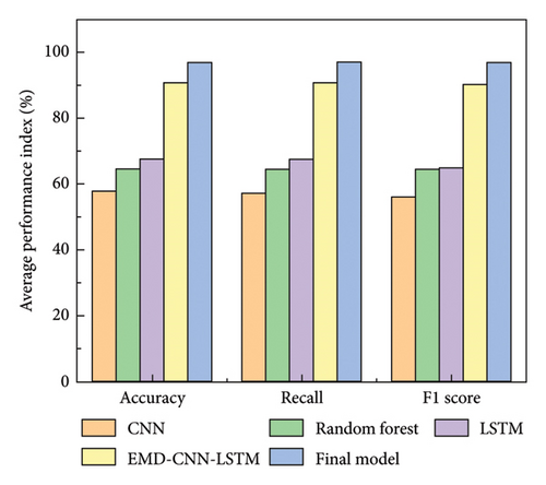
As shown in Table 4 and Figure 13, the proposed model outperforms others across key metrics. It achieves the highest Accuracy of 0.9654, significantly surpassing EMD–CNN–LSTM (0.9074), LSTM (0.6763), Random Forest (0.6454), and CNN (0.5778). The model also improves Recall, outperforming CNN by 0.3904, LSTM by 0.2877, EMD–CNN–LSTM by 0.0561, and Random Forest by 0.3178. For the F1-Score, it reaches 0.9623, well above CNN (0.5616), LSTM (0.6480), EMD–CNN–LSTM (0.9027), and Random Forest (0.6452). The bar chart shows that CNN performs the worst across all metrics, with average values below 60%. Random Forest shows slight improvement at around 64% due to its reliance on handcrafted features. LSTM improves to around 67% for Accuracy and Recall, but its F1-Score is lower. EMD–CNN–LSTM, combining EMD preprocessing and CNN–LSTM, boosts all metrics above 90%. The final model excels, achieving over 96% in Accuracy, Recall, and F1-Score, thanks to the global feature modeling of the multihead self-attention mechanism and the optimizations from the BiLSTM and multiscale feature fusion module. Overall, the model’s performance improves with increasing architectural complexity and enhanced feature extraction.

A confusion matrix was used to further determine which faults were misclassified by the proposed model, providing a visualization of the fault detection results. The EMD–CNN–LSTM neural network optimized by multihead self-attention mechanism is visualized with the Random Forest classification results, as shown in Figure 14.

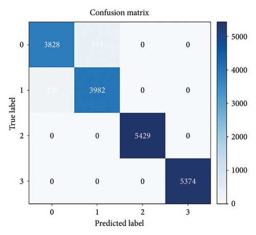
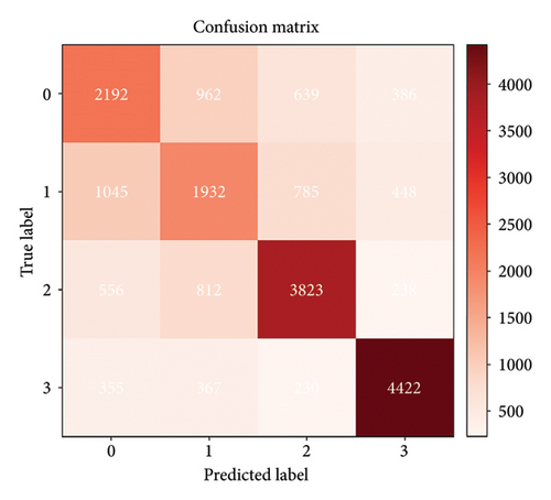
As shown in Figure 14, the proposed model outperforms the traditional Random Forest model by more effectively extracting data features and maximizing the identification of distinctive characteristics across different fault types. For the normal and loosening categories, where the feature differences are relatively small, both models exhibited some misclassification. The multihead self-attention mechanism-optimized EMD–CNN–LSTM neural network misclassified 228 normal samples as loosening and 351 loosening samples as normal. In contrast, the Random Forest model misclassified 1061 and 1774 samples, respectively. This indicates that the proposed model extracts features more comprehensively, resulting in significantly better performance than Random Forest.

4.2.3. Layer-By-Layer Visualization of Model Classification

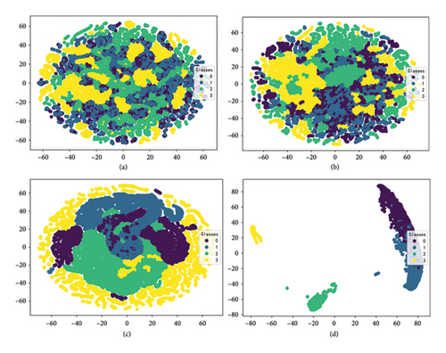
To better understand the model structure and training process, this study visualizes the feature extraction capability of each layer and analyzes the interlayer relationships in the deep network. The T-stochastic neighbor embedding (T-SNE) algorithm is used for dimensionality reduction and visualization of the output features at each layer. As shown in Figure 15(a), the input data are initially cluttered with no clear classification. After passing through the attention mechanism layer (Figure 15(b)), some features are effectively separated and aggregated, but complex features with different time frequencies and scales remain mixed. These features are further refined in the CNN and LSTM layers. Figure 15(c) shows that local features are effectively extracted in the CNN and pooling layers, though some features are still not fully separated. Finally, after the LSTM layer (Figure 15(d)), fault features are clearly extracted and classified, with only a small overlap remaining. Overall, the model successfully learns fault features and performs effective diagnosis and classification.

5. Discussion

5.1. Analysis of Model Performance

5.1.1. Reasons for Performance Enhancement

From Table 4 and Figure 13, it is clear that our proposed method significantly outperforms other algorithms, achieving an F1-Score of 0.9623. This improvement is due to the multihead self-attention mechanism, which effectively captures both global dependencies and local features, integrating time and spatial information to enhance the model’s ability to recognize long-range dependencies. In comparison, CNN performs the worst because it relies solely on spatial feature extraction, making it less effective for complex time-series and multiclass fault data and sensitive to high-frequency noise. Random Forest performs better but is limited by fixed handcrafted features, hindering its ability to capture temporal dependencies. LSTM performs well for time modeling but struggles with spatial feature extraction and is affected by gradient issues. The EMD–CNN–LSTM model improves performance significantly, with EMD preprocessing extracting time–frequency features, and the combination of CNN and LSTM enhancing spatial-temporal feature modeling.

Figure 14 shows that the proposed model correctly classifies all samples for each fault category, especially for rough contact faults, demonstrating its strong time and spatial feature extraction capabilities. It also outperforms Random Forest in diagnostic accuracy. For misalignment faults, the model achieves perfect classification, showcasing its powerful deep feature extraction ability.

5.1.2. Statistical Significance of Model Performance Improvement

An independent sample t-test was conducted to determine whether the performance differences between models were statistically significant, ensuring that the observed performance improvement of the model was not due to chance. The performance index of the final model was compared with those of other models, and the detailed results are presented in Table 5.

Table 5. Statistical significance analysis of performance differences between the proposed model and comparative models.

Model	T-statistic	p value
CNN	80.5611	8.9043 × 10⁻⁵
LSTM	31.7740	8.8625 × 10⁻⁴
EMD–CNN–LSTM	32.5942	2.9951 × 10⁻⁵
Random Forest	344.7944	7.5447 × 10⁻⁶

The t-test results in Table 5 indicate that there is a significant difference between the final model and other models, with all p values being less than 0.001, confirming the statistical significance of the performance improvement of the final model. Compared with LSTM and EMD–CNN–LSTM, the p values are much smaller than 0, and the t-statistics exceed 30, indicating that the improvements brought by the final model are substantial. For Random Forest, the t-statistics and p values further highlight the significant performance difference. In summary, combining Table 5 with Table 4 and Figure 13, the results confirm the significant performance improvement of the final model.

5.2. Analysis of Different Data Decomposition Methods

Further validation of the impact of different signal decomposition methods on the proposed model involved applying VMD to decompose the raw torque data and integrating it into the model. Building on previous studies of VMD in fault diagnosis [53], the fault diagnosis performance was evaluated with the number of modes K set to 6 and 10, respectively. The confusion matrices for both cases are presented in Figure 16.

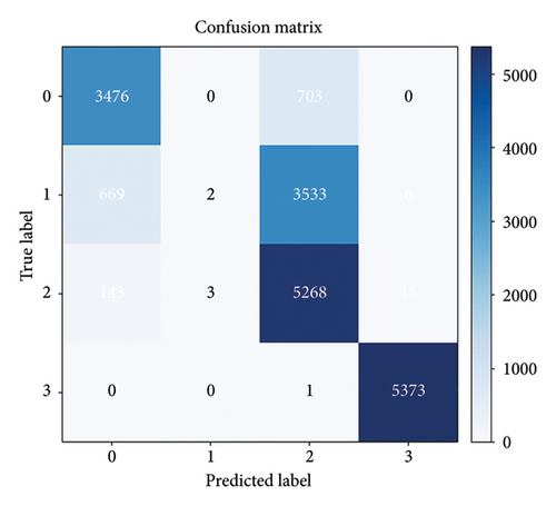
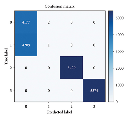
As shown in Figure 16, both VMD schemes with K = 6 and K = 10 failed to distinguish normal from loosening, resulting in significant misclassification. When K = 6, the test Accuracy was 0.7357, the Recall was 0.7006, and the F1-Score was 0.6314, with frequent confusion between fault types. Increasing the number of modes to K = 10 slightly improved Accuracy, Recall, and F1-Score to 0.7806, 0.7499, and 0.6663, but the issue of misclassification, especially between normal and loosening, persisted. Combined with Table 4, it can be seen that the use of the VMD method failed to effectively extract the fine-grained features crucial for distinguishing between different fault types. In contrast, EMD, through its adaptive decomposition approach, was able to better capture time–frequency features, thereby improving the overall performance of the model. Therefore, although VMD has certain advantages in some applications, its performance is clearly inferior to EMD in this task and failed to effectively improve fault diagnosis accuracy.

5.3. Analysis of Model Robustness and Scenario Applications

In the field of fault diagnosis, avoiding noise interference and achieving robust fault detection is crucial for multiscenario applications. The proposed model was tested using the 12 kHz drive-end data from the CWRU dataset [54] under various operating conditions, including 0 HP, 1 HP, 2 HP, and 3 HP, to validate its robustness. The test results in Table 6 indicate that the model achieved accuracies of 97.50%, 95.56%, 94.67%, and 97.33% under these conditions. These findings demonstrate that the model is not only suitable for coupling monitoring of printing equipment but also widely applicable to fault monitoring of key components in other industrial devices, such as spindle drive systems and conveyor belt couplings in machine tools. In future applications, combining high-precision sensors, advanced filtering techniques, and the model’s real-time inference capabilities is expected to significantly enhance the intelligent diagnostic level of equipment in these scenarios.

Table 6. Performance index under different operating conditions in the CWRU dataset.

Operating condition (HP)	Accuracy (%)	Recall (%)	F1-Score (%)
0	97.50	97.14	97.14
1	95.56	94.81	94.93
2	94.67	94.50	94.23
3	97.33	97.40	97.28

5.4. Model Limitations and Improvement Directions

Despite achieving strong classification performance, the proposed EMD–CNN–BiLSTM model optimized with multihead self-attention has some limitations. It struggles in scenarios with minimal feature differences, such as distinguishing between normal and loosening categories, where fine-grained feature extraction is insufficient, leading to misclassification. Moreover, the model has 439,078 parameters in total, with a significant portion coming from the multihead self-attention (68,864 parameters), BiLSTM layers (263,168 parameters), and convolutional layers (98,432 parameters). While these components improve feature extraction, they also result in high computational cost and memory usage, which could limit its deployment in resource-constrained environments, like fault diagnosis in industrial production lines.

Addressing these issues involves enhancing feature extraction through deeper CNNs or techniques such as pyramid pooling or dilated convolutions to capture finer features. High computational cost and memory usage can be mitigated by employing model compression, pruning, or lightweight architectures such as MobileNet or EfficientNet. These approaches improve feature extraction while reducing computational complexity, making the model more suitable for resource-constrained environments such as industrial production lines.

6. Conclusion

A coupling fault diagnosis model is established based on the optimized EMD–CNN–BiLSTM neural network. Abnormal fluctuations and amplitude changes of torque signals are found by collecting and analyzing different fault data signals of coupling.

Comparing the proposed model with the CNN, the LSTM, and the Random Forest, the proposed model effectively captures the feature information in the fault signals and achieves accurate diagnosis of different fault types. The method improves 40.07%, 31.43%, and 31.71% in F1-Score. The multihead self-attention is introduced to further enhance the expressive ability of the model. After the input data pass through the attention mechanism layer, a portion of the features are effectively separated and aggregated. These indicate that the attention mechanism layer is able to extract fault features at different scales. After the LSTM layer, the fault feature extraction and classification are very obvious. The model effectively learns the features of different faults and realizes the goal of diagnosis and classification.

Conflicts of Interest

The authors declare no conflicts of interest.

Funding

This work was supported by the R&D Program of Beijing Municipal Education Commission (KM202410015004), Doctoral Research Startup Fund of Beijing Institute of Graphic Communication (27170124032), and BIGC Project (Ec202301).

Open Research

Data Availability Statement

The data used to support the findings of this study are available on request from the corresponding author.

References

1 Lu Z. Y., Wang X. D., Hou L., Chen Y. S., and Li H. L., Dynamic Response Analysis for the Aero-Engine Dual-Rotor-Bearing System with Flexible Coupling Misalignment Faults, Journal of Vibroengineering. (2018) 20, no. 5, 2012–2026, https://doi.org/10.21595/jve.2017.18553, 2-s2.0-85051665178.
10.21595/jve.2017.18553
Google Scholar
2 Xu Z., Hu Y., Chen Q., Zheng Z., Zhang J., and Wang H., Design and Analysis of the Dual Motor Coupling Drive System for Electric Vehicle, International Journal of Vehicle Design. (2022) 89, no. 3/4, 326–347, https://doi.org/10.1504/ijvd.2022.10053875.
10.1504/IJVD.2022.10053875
Web of Science® Google Scholar
3 Ma L., Zhang J. H., Lin J. W., Wang J., and Lu X., Dynamic Analysis of Rolling Bearing Rotor System with Extruded Oil Film Damper under Misalignment Fault, Journal of Zhejiang University-Science. (2016) 17, no. 08, 614–631.
10.1631/jzus.A1500111
Google Scholar
4 Mei Q. and Lin I., Analysis and Experimental Research on Dynamic Characteristics of Elastic Coupling, Journal of Vibration and Shock. (2008) 6, 128–131+192.
Google Scholar
5 Li C., Research and Implementation of PCA-SVM Based Coupling Fault Detection of Gluing Machine, 2022, South China University of Technology.
Google Scholar
6 Li G. Y., Wang S. B., and Chen X. F., Fault Diagnosis of Wind Turbine Coupling Loosening Based on Adaptive EEMD, Vibration, Test & Diagnosis. (2022) 42, no. 02, 292–298.
Google Scholar
7 Xuan Y., He L., and Liao J., Vibration Analysis of Misalignment Failure of Hydraulic Pump Unit with Plum Blossom-Shaped Flexible Coupling, Journal of National University of Defense Technology. (2019) 41, no. 06, 94–99.
Google Scholar
8 dos Reis Farias M., Koornneef L. R., Vaz Pinto L. A., and R Troyman A. C., Faults Prevention for the Gear Coupling of the Azimuth Thruster L-Drive through a Study of Shaft Alignment Measurements, Engineering Failure Analysis. (2023) 152, https://doi.org/10.1016/j.engfailanal.2023.107504.
10.1016/j.engfailanal.2023.107504
Google Scholar
9 Hujare D. P. and Karnik M. G., Vibration Responses of Parallel Misalignment in Al Shaft Rotor Bearing System with Rigid Coupling, Materials Today: Proceedings. (2018) 5, no. 11, 23863–23871, https://doi.org/10.1016/j.matpr.2018.10.178, 2-s2.0-85058377302.
10.1016/j.matpr.2018.10.178
CAS Google Scholar
10 Chandra M. and Sekhar A. S., Detection and Monitoring of Coupling Misalignment in Rotors Using Torque Measurements, Measurement. (2015) 61, 111–122, https://doi.org/10.1016/j.measurement.2014.10.031, 2-s2.0-84910652595.
10.1016/j.measurement.2014.10.031
Web of Science® Google Scholar
11 Guo Y., Lambert S., Wallen R., Errichello R., and Keller J., Theoretical and Experimental Study on Gear-Coupling Contact and Loads Considering Misalignment, Torque, and Friction Influences, Mechanism and Machine Theory. (2016) 98, 242–262, https://doi.org/10.1016/j.mechmachtheory.2015.11.015, 2-s2.0-84955455307.
10.1016/j.mechmachtheory.2015.11.015
Web of Science® Google Scholar
12 Jiang X. J., Zhu Y. S., Hong J., Chen X., and Zhang Y. Y., Investigation into the Loosening Mechanism of Bolt in Curvic Coupling Subjected to Transverse Loading, Engineering Failure Analysis. (2013) 32, 360–373, https://doi.org/10.1016/j.engfailanal.2013.04.005, 2-s2.0-84877879424.
10.1016/j.engfailanal.2013.04.005
Web of Science® Google Scholar
13 Zhang Q. F., Zhang C. H., Zhao Z. J., and Wu F., Analysis of Loosening of Tooth Coupling Connection of a Crane Hoisting Mechanism, Equipment Management & Maintenance. (2017) 8, 68–69.
Google Scholar
14 Almasoudi F. M., Enhancing Power Grid Resilience through Real-Time Fault Detection and Remediation Using Advanced Hybrid Machine Learning Models, Sustainability. (2023) 15, no. 10, https://doi.org/10.3390/su15108348.
10.3390/su15108348
Web of Science® Google Scholar
15 Xiang L., Wang P. H., Yang X., Hu A., and Su H., Fault Detection of Wind Turbine Based on SCADA Data Analysis Using CNN and LSTM with Attention Mechanism, Measurement. (2021) 175, https://doi.org/10.1016/j.measurement.2021.109094.
10.1016/j.measurement.2021.109094
Web of Science® Google Scholar
16 Vos K., Peng Z. X., Jenkins C., Shahriar M. R., Borghesani P., and Wang W., Vibration-based Anomaly Detection Using LSTM/SVM Approaches, Mechanical Systems and Signal Processing. (2022) 169, https://doi.org/10.1016/j.ymssp.2021.108752.
10.1016/j.ymssp.2021.108752
Web of Science® Google Scholar
17 Zhang J. X., Zhang M., Feng Z. M. et al., Gated Recurrent Unit-Enhanced Deep Convolutional Neural Network for Real-Time Industrial Process Fault Diagnosis, Process Safety and Environmental Protection. (2023) 175, 129–149, https://doi.org/10.1016/j.psep.2023.05.025.
10.1016/j.psep.2023.05.025
CAS Web of Science® Google Scholar
18 Zhang S., Zhu X., Anduv B., Jin X., and Du Z., Fault Detection and Diagnosis for the Screw Chillers Using Multi-Region XGBoost Model, Science and Technology for the Built Environment. (2021) 27, no. 5, 608–623, https://doi.org/10.1080/23744731.2021.1877966.
10.1080/23744731.2021.1877966
Web of Science® Google Scholar
19 Jalayer M., Orsenigo C., and Vercellis C., Fault Detection and Diagnosis for Rotating Machinery: A Model Based on Convolutional LSTM, Fast Fourier and Continuous Wavelet Transforms, Computers in Industry. (2021) 125, https://doi.org/10.1016/j.compind.2020.103378.
10.1016/j.compind.2020.103378
Web of Science® Google Scholar
20 Xue M., Yan H. C., Wang M., Shen H., and Shi K. B., LSTM-based Intelligent Fault Detection for Fuzzy Markov Jump Systems and its Application to Tunnel Diode Circuits, IEEE Transactions on Circuits and Systems II: Express Briefs. (2022) 69, no. 3, 1099–1103, https://doi.org/10.1109/tcsii.2021.3092627.
10.1109/tcsii.2021.3092627
Web of Science® Google Scholar
21 Zhi Z., Liu L. S., Liu D. T., and Hu C., Fault Detection of the Harmonic Reducer Based on CNN-LSTM with a Novel Denoising Algorithm, IEEE Sensors Journal. (2022) 22, no. 3, 2572–2581, https://doi.org/10.1109/jsen.2021.3137992.
10.1109/JSEN.2021.3137992
Web of Science® Google Scholar
22 Attouri K., Mansouri M., Hajji M., Kouadri A., Bouzrara K., and Nounou H., Wind Power Converter Fault Diagnosis Using Reduced Kernel PCA-Based BiLSTM, Sustainability. (2023) 15, no. 4, https://doi.org/10.3390/su15043191.
10.3390/su15043191
Web of Science® Google Scholar
23 Yan X. Y., Guan T., Fan K. X., and Sun Q., Novel Double Layer BiLSTM Minor Soft Fault Detection for Sensors in Air-Conditioning System with KPCA Reducing Dimensions, Journal of Building Engineering. (2021) 44, https://doi.org/10.1016/j.jobe.2021.102950.
10.1016/j.jobe.2021.102950
Web of Science® Google Scholar
24 Nacer S. M., Nadia B., Abdelghani R., and Mohamed B., A Novel Method for Bearing Fault Diagnosis Based on BiLSTM Neural Networks, The International Journal of Advanced Manufacturing Technology. (2023) 125, no. 3-4, 1477–1492, https://doi.org/10.1007/s00170-022-10792-1.
10.1007/s00170-022-10792-1
Web of Science® Google Scholar
25 Song B. Y., Liu Y. Y., Fang J. Z., Liu W. B., Zhong M. Y., and Liu X. H., An Optimized CNN-BiLSTM Network for Bearing Fault Diagnosis under Multiple Working Conditions with Limited Training Samples, Neurocomputing. (2024) 574, https://doi.org/10.1016/j.neucom.2024.127284.
10.1016/j.neucom.2024.127284
Web of Science® Google Scholar
26 Liu J. F., Failure Analysis and Countermeasure Research of Gate Opener Coupling of Urban Reservoir, Water Resources Science and Economics. (2023) 29, no. 12, 155–160.
Google Scholar
27 Jiao Z. S., Research on Fatigue Factor Hidden Anomaly Detection and Fault Diagnosis Method Based on LSTM, 2022, Hebei University of Technology.
Google Scholar
28 Civera M. and Surace C., A Comparative Analysis of Signal Decomposition Techniques for Structural Health Monitoring on an Experimental Benchmark, Sensors. (2021) 21, no. 5, https://doi.org/10.3390/s21051825.
10.3390/s21051825
Web of Science® Google Scholar
29 He X. Z., Zhou X. Q., Yu W. N., Hou Y. X., and Mechefske C. K., Adaptive Variational Mode Decomposition and its Application to Multi-Fault Detection Using Mechanical Vibration Signals, ISA Transactions. (2021) 111, 360–375, https://doi.org/10.1016/j.isatra.2020.10.060.
10.1016/j.isatra.2020.10.060
PubMed Web of Science® Google Scholar
30 Li Y., Zhou J., Li H., Meng G., and Bian J., A Fast and Adaptive Empirical Mode Decomposition Method and its Application in Rolling Bearing Fault Diagnosis, IEEE Sensors Journal. (2023) 23, no. 1, 567–576, https://doi.org/10.1109/jsen.2022.3223980.
10.1109/JSEN.2022.3223980
Web of Science® Google Scholar
31 Shi Y. P., Li B., Li L., Liu T. K., Du X., and Wei X., Automatic Non-contact Grinding Surface Roughness Measurement Based on Multi-Focused Sequence Images and CNN, Measurement Science and Technology. (2024) 35, no. 3, https://doi.org/10.1088/1361-6501/ad1804.
10.1088/1361-6501/ad1804
PubMed Web of Science® Google Scholar
32 Zhou C., Zhou C. Z., Zhu H. Q., and Liu T. H., AIR-CNN: a Lightweight Automatic Image Rectification CNN Used for Barrel Distortion, Measurement Science and Technology. (2024) 35, no. 4, https://doi.org/10.1088/1361-6501/ad1979.
10.1088/1361-6501/ad1979
PubMed Web of Science® Google Scholar
33 Yuan Z. R., Zhang P. L., Ming B., Zheng X. B., and Tian L., Joint Forecasting Method of Wind and Solar Outputs Considering Temporal and Spatial Correlation, Sustainability. (2023) 15, no. 19, https://doi.org/10.3390/su151914628.
10.3390/su151914628
Web of Science® Google Scholar
34 Fu G. H., Wei Q. J., Yang Y. S., and Li C. F., Bearing Fault Diagnosis Based on CNN-BiLSTM and Residual Module, Measurement Science and Technology. (2023) 34, no. 12, https://doi.org/10.1088/1361-6501/acf598.
10.1088/1361-6501/acf598
Web of Science® Google Scholar
35 Kavianpour P., Kavianpour M., Jahani E., and Ramezani A., A CNN-BiLSTM Model with Attention Mechanism for Earthquake Prediction, The Journal of Supercomputing. (2023) 79, no. 17, 19194–19226, https://doi.org/10.1007/s11227-023-05369-y.
10.1007/s11227-023-05369-y
Web of Science® Google Scholar
36 Shi X. B., Li B. J., Wang W., Qin Y., Wang H., and Wang X., Classification Algorithm for Electroencephalogram-Based Motor Imagery Using Hybrid Neural Network with Spatio-Temporal Convolution and Multi-Head Attention Mechanism, Neuroscience. (2023) 527, 64–73, https://doi.org/10.1016/j.neuroscience.2023.07.020.
10.1016/j.neuroscience.2023.07.020
CAS PubMed Web of Science® Google Scholar
37 Lan T. H., Zhang X. J., Qu D. Y., Yang Y. F., and Chen Y. C., Short-term Traffic Flow Prediction Based on the Optimization Study of Initial Weights of the Attention Mechanism, Sustainability. (2023) 15, no. 2, https://doi.org/10.3390/su15021374.
10.3390/su15021374
Web of Science® Google Scholar
38 Xie J. X., Liang Y. C., Sun B., Pu Y. W., Wang M. Q., and Qin Z. F., Recurrent Neural Network Based on Attention Mechanism in Prediction of Glass Forming Ability by Element Proportion, Materials Today Communications. (2024) 38, https://doi.org/10.1016/j.mtcomm.2023.107853.
10.1016/j.mtcomm.2023.107853
PubMed Web of Science® Google Scholar
39 Dong L., Wang H. D., and Lou J. K., An Attention Mechanism Model Based on Positional Encoding for the Prediction of Ship Maneuvering Motion in Real Sea State, Journal of Marine Science and Technology. (2024) 29, no. 1, 136–152, https://doi.org/10.1007/s00773-023-00978-x.
10.1007/s00773-023-00978-x
Web of Science® Google Scholar
40 Cao Y., Hou X. L., and Chen N., Short-term Forecast of OD Passenger Flow Based on Ensemble Empirical Mode Decomposition, Sustainability. (2022) 14, https://doi.org/10.3390/su14148562.
10.3390/su14148562
Web of Science® Google Scholar
41 Agarwal P., Gonzalez J. I. M., Elkamel A., and Budman H., Hierarchical Deep LSTM for Fault Detection and Diagnosis for a Chemical Process, Processes. (2022) 10, no. 12, https://doi.org/10.3390/pr10122557.
10.3390/pr10122557
Web of Science® Google Scholar
42 Chen Y. F. and Fu Z. H., Multi-step Ahead Forecasting of the Energy Consumed by the Residential and Commercial Sectors in the united states Based on a Hybrid CNN-BiLSTM Model, Sustainability. (2023) 15, no. 3, https://doi.org/10.3390/su15031895.
10.3390/su15031895
Web of Science® Google Scholar
43 Dai H. B., Huang G. Q., Zeng H. B., and Yang F., PM2.5 Concentration Prediction Based on Spatiotemporal Feature Selection Using XGBoost-MSCNN-GA-LSTM, Sustainability. (2021) 13, no. 21, https://doi.org/10.3390/su132112071.
10.3390/su132112071
Web of Science® Google Scholar
44 Yan J. S., Liu Y. Q., and Ren X. Y., An Early Fault Detection Method for Wind Turbine Main Bearings Based on Self-Attention GRU Network and Binary Segmentation Changepoint Detection Algorithm, Energies. (2023) 16, no. 10, https://doi.org/10.3390/en16104123.
10.3390/en16104123
PubMed Web of Science® Google Scholar
45 Li S. F., Xu Y. H., Jiang W., Zhao K. J., and Liu W., A Modular Fault Diagnosis Method for Rolling Bearing Based on Mask Kernel and Multi-Head Self-Attention Mechanism, Transactions of the Institute of Measurement and Control. (2024) 46, no. 5, 899–912, https://doi.org/10.1177/01423312231188777.
10.1177/01423312231188777
Web of Science® Google Scholar
46 Vaswani A., Shazeer N., Parmar N. et al., Attention Is All You Need, Advances in Neural Information Processing Systems. (2017) 30, 5998–6008.
Google Scholar
47 Szegedy C., Liu W., Jia Y. et al., Going Deeper with Convolutions, 2015 IEEE Conference on Computer Vision and Pattern Recognition (CVPR). (2015) 1, 1–9, https://doi.org/10.1109/cvpr.2015.7298594, 2-s2.0-84937522268.
10.1109/cvpr.2015.7298594
Google Scholar
48 Bingham G., Macke W., and Miikkulainen R., Evolutionary Optimization of Deep Learning Activation Functions, Proceedings of the 2020 Genetic and Evolutionary Computation Conference (GECCO20), July 2020, Cancún, Mexico, 289–296, https://doi.org/10.1145/3377930.3389841.
10.1145/3377930.3389841
Google Scholar
49 Zhang Y. and Yang Q., A Survey on Multi-Task Learning, IEEE Transactions on Knowledge and Data Engineering. (2022) 34, no. 12, 5586–5609, https://doi.org/10.1109/tkde.2021.3070203.
10.1109/TKDE.2021.3070203
Web of Science® Google Scholar
50 Zheng Y. C., Iwana B. K., and Uchida S., Mining the Displacement of Max-Pooling for Text Recognition, Pattern Recognition. (2019) 93, 558–569, https://doi.org/10.1016/j.patcog.2019.05.014, 2-s2.0-85065551518.
10.1016/j.patcog.2019.05.014
Web of Science® Google Scholar
51 Srivastava N., Hinton G., Krizhevsky A., Sutskever I., and Salakhutdinov R., Dropout: a Simple Way to Prevent Neural Networks from Overfitting, Journal of Machine Learning Research. (2014) 15, no. 1, 1929–1958.
Web of Science® Google Scholar
52 Cerrada M., Zurita G., Cabrera D., Sánchez R. V., Artés M., and Li C., Fault Diagnosis in Spur Gears Based on Genetic Algorithm and Random Forest, Mechanical Systems and Signal Processing. (2016) 70-71, 87–103, https://doi.org/10.1016/j.ymssp.2015.08.030, 2-s2.0-84961051737.
10.1016/j.ymssp.2015.08.030
Web of Science® Google Scholar
53 Zhou J. B., Xiao M. H., Niu Y., and Ji G. J., Rolling Bearing Fault Diagnosis Based on WGWOA-VMD-SVM, Sensors. (2022) 22, no. 16, https://doi.org/10.3390/s22166281.
10.3390/s22166281
Web of Science® Google Scholar
54 Bearings Data Center, Seeded Fault Test Data, 2024, Case Western Reserve University.
Google Scholar

All articles

An Improved Fault Diagnosis Method and Its Application in Compound Fault Diagnosis for Paper Delivery Structure Coupling

Abstract

1. Introduction

2. Data Resource

2.1. Data Preprocessing

2.2. Data Details

3. Methods

3.1. Data Standardization

3.2. EMD

3.3. Fault Diagnosis Classification Model

3.3.1. BiLSTM Neural Network Model

3.3.2. CNN

3.3.3. Multihead Self Attention Mechanism

3.3.4. Optimized EMD–CNN–BiLSTM Model With Multihead Self-Attention Mechanism

3.4. Performance Index

4. Fault Detection Results Analysis

4.1. Enhanced Representation of Data Features

4.2. Validation of Fault Detection Model Effectiveness

4.2.1. Model Parameters

4.2.2. Model Test Results

4.2.3. Layer-By-Layer Visualization of Model Classification

5. Discussion

5.1. Analysis of Model Performance

5.1.1. Reasons for Performance Enhancement

5.1.2. Statistical Significance of Model Performance Improvement

5.2. Analysis of Different Data Decomposition Methods

5.3. Analysis of Model Robustness and Scenario Applications

5.4. Model Limitations and Improvement Directions

6. Conclusion

Conflicts of Interest

Funding

Open Research

Data Availability Statement

References

Figures

References

Related

Information