Volume 2025, Issue 1 1904885

Research Article

Open Access

A Fault Diagnosis Method for Typical Failures of Marine Diesel Engines Based on Multisource Information Fusion

Rongjun Jiang

School of Mechanical and Electronic Engineering , Quanzhou University of Information Engineering , Quanzhou , 362000 , China

Search for more papers by this author

Shunhua Ou,

Corresponding Author

Shunhua Ou

[email protected]

orcid.org/0000-0002-5815-1472

School of Naval Architecture , Ocean and Energy Power Engineering , Wuhan University of Technology , Wuhan , 430063 , China , whut.edu.cn

Search for more papers by this author

Baoyue Li,

Baoyue Li

orcid.org/0009-0009-4768-2903

School of Naval Architecture , Ocean and Energy Power Engineering , Wuhan University of Technology , Wuhan , 430063 , China , whut.edu.cn

Search for more papers by this author

Wenwu Liu,

Wenwu Liu

School of Mechanical and Electronic Engineering , Quanzhou University of Information Engineering , Quanzhou , 362000 , China

Search for more papers by this author

Bingxin Cao,

Bingxin Cao

School of Naval Architecture , Ocean and Energy Power Engineering , Wuhan University of Technology , Wuhan , 430063 , China , whut.edu.cn

Search for more papers by this author

Yonghua Yu,

Yonghua Yu

School of Naval Architecture , Ocean and Energy Power Engineering , Wuhan University of Technology , Wuhan , 430063 , China , whut.edu.cn

Search for more papers by this author

Rongjun Jiang,

Rongjun Jiang

School of Mechanical and Electronic Engineering , Quanzhou University of Information Engineering , Quanzhou , 362000 , China

Search for more papers by this author

Shunhua Ou,

Corresponding Author

Shunhua Ou

[email protected]

orcid.org/0000-0002-5815-1472

School of Naval Architecture , Ocean and Energy Power Engineering , Wuhan University of Technology , Wuhan , 430063 , China , whut.edu.cn

Search for more papers by this author

Baoyue Li,

Baoyue Li

orcid.org/0009-0009-4768-2903

School of Naval Architecture , Ocean and Energy Power Engineering , Wuhan University of Technology , Wuhan , 430063 , China , whut.edu.cn

Search for more papers by this author

Wenwu Liu,

Wenwu Liu

School of Mechanical and Electronic Engineering , Quanzhou University of Information Engineering , Quanzhou , 362000 , China

Search for more papers by this author

Bingxin Cao,

Bingxin Cao

School of Naval Architecture , Ocean and Energy Power Engineering , Wuhan University of Technology , Wuhan , 430063 , China , whut.edu.cn

Search for more papers by this author

Yonghua Yu,

Yonghua Yu

School of Naval Architecture , Ocean and Energy Power Engineering , Wuhan University of Technology , Wuhan , 430063 , China , whut.edu.cn

Search for more papers by this author

First published: 07 May 2025

https://doi.org/10.1155/vib/1904885

Academic Editor: Andrzej Katunin

Share a link

Email
Wechat
Bluesky

Abstract

Due to the fact that different components of a diesel engine may exhibit the same fault phenomenon, leading to a low fault identification rate caused by one effect with multiple causes, this paper acquires multiple thermodynamic parameters under various fault conditions through models. The k-nearest neighbors mutual information (KNN-MI) method is used to calculate the correlation between different thermodynamic parameters, eliminate strong correlation coefficients, and select thermodynamic parameters with low correlation for fault diagnosis. Comprehensively comparing the downscaling effects of the four different downscaling methods, the data after downscaling by the t-SNE are characterized by a smaller distance within the class, a larger distance between the classes, and a better classification effect, which is used for the downscaling of the fusion of the screened thermal parameters and vibration feature parameters, and finally, the feature fusion method is used. An accuracy rate of 98.7% was achieved and compared with the fault diagnosis method based on a single signal of vibration. The fusion of multisource information can effectively distinguish between different fault categories and improve the accuracy of diesel engine fault identification.

1. Introduction

During the actual operation of a diesel engine, the reciprocating motion of the piston cylinder is its main form of movement, accompanied by the rotating motion of the crankshaft, which outputs power to mechanical equipment. The impact force generated by the piston movement, as well as the unbalanced inertial force produced by the sequential work of multiple cylinders with the change of the crankshaft angle, makes the fault form of the diesel engine different from other reciprocating mechanisms. In addition, the complex and numerous mechanical parts in the diesel engine work together, the system itself has a large amount of noise, and some characteristic indicators are in a state of cyclical fluctuation, which adds obstacles to the fault analysis of the engine. At the same time, different parts of the fault may show the same fault phenomenon; for example, when the injector fails, the cylinder head vibration data displayed may be similar to those of other parts when they fail, which is the so-called one effect with multiple causes [1]. The abovementioned factors lead to the difficulty in achieving the general level of mechanical fault diagnosis in terms of accuracy and speed for diesel engine fault diagnosis. In addition, diesel engines are usually in a harsh working environment, with numerous on-site noises and greater interference in signal transmission, making effective information features easy to be submerged [2]. Therefore, under actual environmental conditions, it is difficult to achieve accurate fault diagnosis of the injector based solely on the cylinder head vibration signal.

Therefore, by analyzing, processing, and fusing multiclass sensor information that represents different states of the diesel engine, a more accurate and comprehensive estimation and judgment can be produced than single sensor information. This paper addresses the complex and diverse causes of diesel engine failures and the low diagnostic identification rate caused by one effect with multiple causes. It uses a multisource information fusion method to fuse and reduce the dimension of cylinder head vibration and thermodynamic parameters, thereby effectively distinguishing different types of diesel engine failures and achieving accurate identification of different types of diesel engine failures.

Multisource information fusion is a signal processing technology that integrates signals from different sources and transforms them into a unified feature information representation [3, 4]. Information fusion can collect information from different angles and sources, providing a more comprehensive state perception, reducing misdiagnosis, and improving diagnostic robustness [5, 6]. By integrating information from multiple sources, it can reduce redundancy, improve information utilization, automate data processing and analysis processes, and improve decision-making efficiency [7, 8].

According to the different levels of information fusion, it can be divided into data layer fusion, feature layer fusion, and decision layer fusion. Feature fusion, as one of the multisource information fusion methods, can greatly reduce the amount of signal processing data compared with data layer fusion and improve computational speed; compared with decision layer fusion, it can avoid conflicts between different decision results [9, 10]. If the obtained various signals are simply merged, on the one hand, it is easy to cause dimensional disaster and increase computational time; on the other hand, not all extracted features are sensitive to faults, and insensitive features will affect the accuracy of the diagnostic model. Therefore, using feature dimensionality reduction algorithms, the high-dimensional features formed by merging different signal types are projected into a low-dimensional space, which can not only eliminate redundant features and reduce model computation time but also improve the model’s diagnostic accuracy [11, 12].

Reference [13] proposes an adaptive dynamic weighted hybrid distance-Taguchi method (ADWHD-T) that integrates data from multiple sensors into a single system-level performance indicator, improving fault diagnosis accuracy compared to other methods. Reference [14] proposes a motor fault diagnosis method based on convolutional neural network (CNN) multifeature fusion, which performs multiscale feature extraction and time series fusion on the vibration and current signals of the motor and has higher diagnostic accuracy and stability than single signal input. Reference [15] addresses the challenge of distinguishing between various faults in rotating machinery, which share related vibration characteristics, by proposing a method that fuses vibration and electrical signal data. This method generates a fused decision by weighting and combining the outputs of multiple sensors, effectively detecting various faults within rotating machinery. Reference [16] uses principal component analysis (PCA) to reduce the dimension of the entrance and exit pressure signals measured by the hydraulic directional valve and construct machine learning samples, comparing the XGBoost model with classification and regression tree models and random forest models. The results show that the proposed method can effectively identify valve faults in hydraulic directional valves with high fault diagnosis accuracy.

From the abovementioned literature, it can be seen that multisource information fusion has significant advantages compared to single signal sources in fault diagnosis. Multisource information fusion can effectively distinguish different fault categories and improve fault diagnosis accuracy. However, there are few application cases of multisource information fusion on diesel engines. The current challenges faced by multisource information fusion include data heterogeneity, fusion algorithm selection, computational complexity, real-time requirements, data security, and privacy protection.

2. Acquisition and Analysis of Cylinder Head Vibration Signals for Typical Diesel Engine Faults

2.1. Diesel Engine Cylinder Head Vibration Signal Acquisition

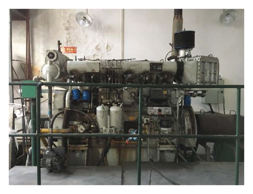
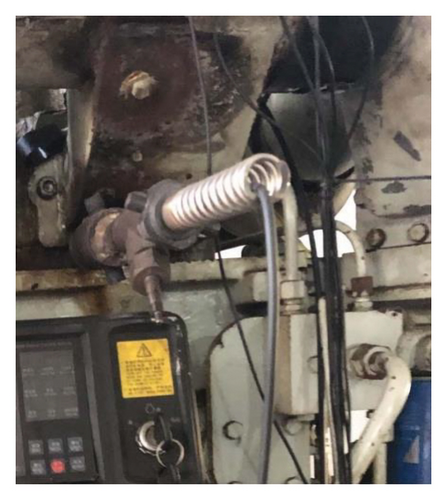
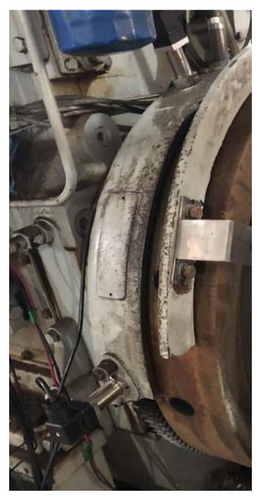
Table 1 shows the main technical parameters of the Z6170 marine diesel engine, and Table 2 shows the relevant parameters of sensors in the acquisition system. Figure 1 shows the test rig of the Z6170 marine medium-speed diesel engine, and Figure 2 shows the layouts of cylinder pressure sensors and speed sensors. A vibration sensor is arranged for each cylinder to measure cylinder head vibration data, a cylinder pressure sensor is arranged for 4# cylinder to measure cylinder pressure, and two speed sensors and a top stop sensor are arranged at the flywheel end to obtain the diesel engine’s speed and top stop signals. Thermal parameter signals are collected by on-board sensors.

Table 1. Main technical parameters of the Z6170 model.

Parameter (unit)	Value
Bore diameter (mm)	170
Cylinder arrangement	Inline
Number of cylinders	6
Compression ratio	14.5
Firing order	1-5-3-6-2-4
Connecting rod length (mm)	480
Rated speed (r/min)	1000

Table 2. Main technical parameters of the Z6170 model.

Measuring signal	Sensor model	Signal type	Quantity
Exhaust gas temperature	PT1000	Current signal	6
Turbocharger inlet temperature	PT1000	Current signal	2
Turbocharger outlet temperature	PT1000	Current signal	2
High temperature water	PT100	Current signal	3
Low temperature water temperature	PT100	Current signal	2
Cylinder pressure	Kistler 6052C cylinder pressure sensor	Voltage signal	1
Cylinder head vibration	BW13100 vibration sensor	Voltage signal	6
Upper stop	Magnetoelectric sensor	Rectangular pulse wave voltage signal	1
Speed	Hall sensor	Rectangular pulse wave voltage signal	2

Details are in the caption following the image — **Figure 1**
Open in figure viewer PowerPoint

Z6170 marine medium-speed diesel engine.

To obtain fault samples, with cylinder #1 as the subject, six typical faults were simulated, including misfire, nozzle blockage, fuel injector needle valve wear, exhaust valve leakage, reduction in air valve pressure, and piston ring wear. The fault simulation methodology is shown in Figure 3.

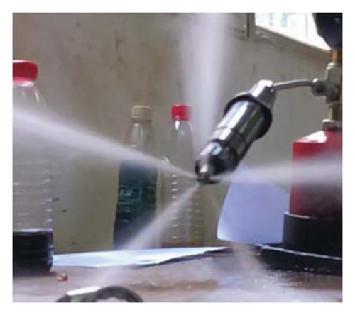
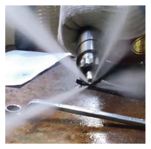
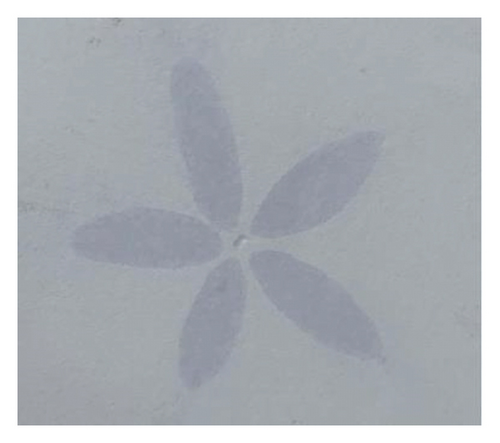
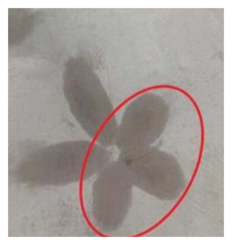
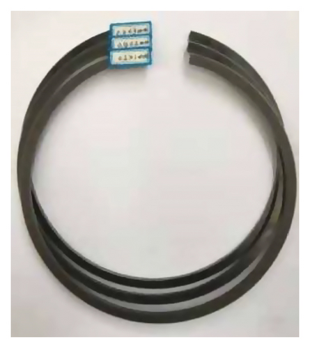
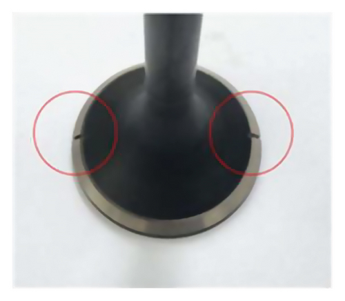
Figure 4 shows the time-domain diagrams of cylinder head vibration data for the normal operation and seven types of faults of the Zibo Diesel Z6170 marine diesel engine. Six common fault types of the diesel engine were simulated through experiments (reduced valve pressure, plugged holes, needle valve wear, exhaust valve leakage, piston ring wear, and single-cylinder misfire), and cylinder head vibration data under different fault conditions were obtained by arranging vibration sensors on the cylinder head of the diesel engine.

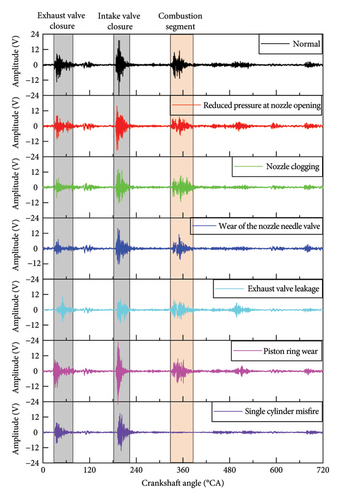
By observing the fluctuation pattern of the cylinder head vibration data in the time domain and comparing the intake and exhaust valve timing and ignition timing of the diesel engine, it can be determined that the cylinder head vibration mainly includes three excitation sources: intake valve closure, exhaust valve closure, and combustion. The intake and exhaust valves exert impact forces on the cylinder head during the closing process, and the fuel in the cylinder exerts impact forces on the cylinder head during the combustion process; hence, the cylinder head vibration time-domain diagram shows three larger vibration amplitudes. Since the fuel injector mainly affects the combustion process inside the cylinder, the faults of the fuel injector can be identified by analyzing the changes in the combustion segment data.

Comparing the time-domain waveform diagrams of the three different types of fuel injector faults in Figure 4 (reduced valve pressure, plugged holes, and needle valve wear), it can be found that there are differences between these three types of faults. For example, the combustion segment peaks of needle valve wear and reduced valve pressure are different; thus, it is possible to identify different types of faults in the same component through data analysis. However, there is a certain similarity between the vibration data of different component faults, such as the similarity in amplitude and combustion duration time-domain waveforms between exhaust valve leakage faults and fuel injector plugging faults, which adds difficulty to identifying different component faults through vibration data and can easily lead to misidentifying exhaust valve leakage faults as fuel injector plugging faults. In addition, the characteristics of single-cylinder misfire faults are very distinct from other faults and are easy to identify. From the measured vibration data, it can be seen that identifying faults between different components solely through the combustion segment data of cylinder head vibration is challenging and requires the combination of other parameters to diagnose faults in different components, thereby improving the accuracy of fault identification.

2.2. Simulation Model Based on AVL Boost

Some thermodynamic parameter sensors of this model are not installed; hence, a simulation calculation method is used to obtain thermodynamic parameters. Taking the Z6170 marine diesel engine as the research object, a thermodynamic parameter model of the diesel engine is established based on the AVL Boost simulation platform. Figure 5 shows the thermodynamic parameter simulation model of the Z6170 diesel engine established using AVL Boost software. In the model, SB1∼SB2 represent system boundaries; TC1 is the exhaust turbocharger; CO1 is the air intercooler; PL1 is the intake manifold; PL2 is the exhaust pipe; TC1 is the turbocharger; CAT1 is the exhaust gas treatment unit; MP is the measurement point; C1 ∼ C6 are cylinders 1 to 6; CL1 is the air filter; 1 ∼ 23 are pipeline connections; MP1 ∼ MP15 are gas state measurement points; J1 ∼ J4 are connecting flanges.

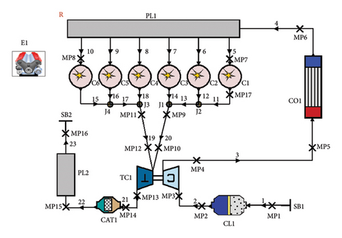
The input parameters required for model construction cover multiple aspects: first, boundary conditions, including environmental temperature, pressure, the flow coefficient, the gas calorific value, and the air-fuel ratio; cylinder parameters, such as cylinder diameter, stroke, connecting rod length, firing order, intake and exhaust valve configuration, as well as combustion and heat release models; in addition, there are structural parameters, which involve basic dimensions, operating state parameters, initial settings, and average mechanical loss pressure. As for the design parameters of each component, they can be obtained from the diesel engine’s user manual or through experimental calibration, while structural parameters come from technical drawings, or are determined through actual measurement or testing.

Table 3 shows the parameter settings for the main boundary conditions and combustion models in the AVL Boost model. The boundary inlet parameters represent the initial conditions of the diesel engine’s intake environment, and the boundary outlet parameters represent the initial conditions of the diesel engine’s exhaust gas outlet environment; the shape parameter m in the single Weber combustion model is a parameter in the VIBE combustion model, which can affect the heat release pattern of the combustion model, and is usually selected based on the fuel type, speed, and injection method of the target engine; the intake and exhaust valve parameters are set according to the parameters of the target engine.

Table 3. Main model parameter settings.

Submodel	Parameter	Value
Boundary conditions	Temperature at boundary inlet SB1 (K)	300
	Pressure at boundary inlet SB1 (MPa)	0.1
	Temperature at boundary outlet SB2 (K)	579
	Pressure at boundary outlet SB2 (MPa)	0.1

Single wiebe combustion model	Fuel injection advance angle (°)	24
Single wiebe combustion model	Shape parameter (m)	1.6

Intake and exhaust valves	Intake valve opening timing (°CA)	BTDC 50
	Exhaust valve opening timing (°CA)	BBDC 50
	Exhaust valve closing timing (°CA)	ATDC 42
	Intake valve closing timing (°CA)	ATDC 50

The relevant parameters in the combustion model can be obtained through design parameters or experimental calibration, and a small number of parameters use empirical values. The single Wiebe model is used to calculate the heat release, and the calculation formula is as follows:

\begin{matrix} \frac{d x}{d α} = \frac{a}{Δ α_{c}} \cdot (m + 1) \cdot y^{m} \cdot \exp (- a \cdot y^{(m + 1)}), \\ d x = \frac{d Q}{Q}, \\ y = \frac{α - α_{0}}{Δ α_{c}} . \end{matrix}

()

In the formula, x is the fraction of fuel mass consumed from the start of combustion to a certain moment; Q is the total heat released by the fuel combustion in each cycle within the cylinder; α is the crankshaft rotation angle; α₀ is the crankshaft rotation angle corresponding to the start of combustion; Δα_c is the combustion duration; m is the shape parameter; a is the completely burned Vibe parameter, a = 6.9.

Integrating the Vibe function of the abovementioned equation yields the fraction of fuel mass burned from the start of combustion to a certain moment, that is, the mass fraction of burned fuel x, as shown in equation (2):

\begin{matrix} x = \int \frac{d x}{d α} \cdot d α = 1 - \exp (- a \cdot y^{(m + 1)}) . \end{matrix}

()

The Woschni 1978 heat transfer model [17] is selected to calculate the convective heat transfer coefficient inside the high-pressure cycle cylinder, and the calculation formula is as follows:

\begin{matrix} α_{w} = 130 \cdot D^{- 0.2} \cdot p_{c}^{0.8} \cdot T_{c}^{- 0.53} \times {[C_{1} \cdot c_{m} + C_{2} \cdot \frac{V_{D} \cdot T_{C, 1}}{P_{C, 1} \cdot V_{C, 1}} \cdot (p_{c} - p_{c, o})]}^{0.8} . \end{matrix}

()

In the formula, D is the cylinder diameter; p_c is the pressure inside the cylinder; T_c is the temperature inside the cylinder; C₁ = 2.28 + 0.308·c_u/c_m; c_m is the average piston speed; cu is the circumferential speed; C₂ = 0.00324; V_D is the displacement per cylinder; T_C,1 is the temperature inside the cylinder when the gas valve is closed; P_C,1 is the pressure inside the cylinder when the gas valve is closed; V_C,1 is the volume of the cylinder when the gas valve is closed; P_C,o is the main engine cylinder pressure.

2.3. Verification of the Simulation Model

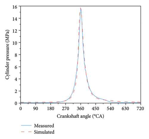
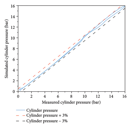
To verify the accuracy of the diesel engine model, bench test data were used to calibrate the simulation results of the model. Figure 6 shows the comparison of simulated and measured cylinder pressure at 50% load and 1000 r/min (there are no more data available to describe the operating conditions of diesel engines), and the results show that the error between simulation and measured cylinder pressure is within 3%, indicating that the model’s calculation accuracy meets the requirements. In addition to cylinder pressure, other simulated parameters were also compared with the test results, as shown in Table 4. The results show that all simulated parameters have an error within 3% compared to the test results, indicating that the model’s calculation accuracy meets the requirements.

Table 4. Comparison of simulation calculations and experimental results at 50% load and 1000 r/min operating conditions.

Name	Experimental data	Computed results	Error (%)
Power (kW)	164.8	168.5	2.2
Temperature after intercooler (K)	314.9	309.8	1.6
Maximum combustion pressure (MPa)	15.6	15.7	0.6
Exhaust temperature before turbine (K)	660.2	652.9	1.1
Exhaust temperature after turbine (K)	638.2	629.4	1.4

By calibrating the simulation results of the model, the accuracy of the model is verified, ensuring that the simulation model meets the application requirements for the simulation analysis of thermodynamic parameter changes under diesel engine fault conditions. This model can be used for the simulation analysis of thermodynamic parameter changes under diesel engine fault conditions, predicting the changes in thermodynamic parameters of the diesel engine under different fault conditions, thereby better achieving fault diagnosis of the diesel engine.

3. Selection of Thermodynamic Parameters Based on Mutual Information (MI)

The various subsystems that make up a diesel engine are closely interrelated, and these relationships result in certain correlations among many thermodynamic parameters. Since thermodynamic parameters with strong correlations contain similar fault information, only one thermodynamic parameter is needed to represent the corresponding fault information. Therefore, to reduce the interference of the selected thermodynamic parameters and improve the accuracy and speed of the fault diagnosis model, it is necessary to use an appropriate method to select thermodynamic parameters, filter out those with low correlations, and eliminate those with strong correlations.

3.1. k-Nearest Neighbors Mutual Information (KNN-MI)

MI is a concept in the information theory that measures the mutual dependence between two random variables. If two variables are independent, their MI is zero; if one variable contains information about another, the MI will be a positive value. MI can be understood as the amount of information one variable contains about another variable, quantifying the information about another variable by reducing the uncertainty of one variable.

In the fields of machine learning and data mining, MI is often used for feature selection, helping to determine which features are most helpful for predicting the target variable. Different assessment methods of MI have their advantages and disadvantages and are suitable for different scenarios and data types.

Combining the characteristics of simulated thermodynamic parameter data, the KNN-MI method is used to calculate the correlation between different thermodynamic parameters. The KNN-MI method is used to calculate the correlation between thermodynamic parameters in the various subsystems that make up the diesel engine and then select thermodynamic parameters with low correlation for fault diagnosis. For example, the correlation between thermodynamic parameters such as pressure, temperature, and flow of the diesel engine can be calculated, and then, parameters with low correlation can be selected for fault diagnosis, which can improve the accuracy and speed of the fault diagnosis model.

The KNN-MI calculation process mainly involves several key mathematical concepts and steps. The following are the main concepts and formulas involved in KNN-MI calculation [18]:

1.
KNN distance: For any two points x_i and x_j, in the dataset, the distance between them can be calculated using Euclidean distance or other distance metrics:
$\begin{matrix} d (x_{i}, x_{j}) = \sqrt{\sum_{k = 1}^{n} {(x_{i k} - x_{j k})}^{2} .} \end{matrix}$ ()
In the formula, x_ik and x_jk are the coordinate values of points x_i and x_j in the kth dimension, respectively.
2.
KNN set: For each point x_i, its KNN set N_k(x_i) is composed of the k points that are closest to it:
$\begin{matrix} N_{k} (x_{i}) = \{x_{j} |d (x_{i}, x_{j}) \leq d (x_{i}, x_{k th - nearest}), j \neq i\} . \end{matrix}$ ()
3.
Local information: For each point, its MI with the KNN set can be estimated by comparing the distribution differences between the original space and the target space. A simplified method for calculating local MI is based on the entropy of histograms:
$\begin{matrix} LMI (x_{i}) = H (X) - \frac{1}{|N_{k} (x_{i})|} \sum_{x_{j} \in N_{k} (x_{i})} H (X |X_{j}) . \end{matrix}$ ()
In the formula, H(X) is the entropy of the original variable X, and H(X|X_j) is the conditional entropy of the variable X given x_i.
4.
Average local MI: For each pair of variables X and Y, the average of the local MI for all points is calculated to estimate the MI between them:
$\begin{matrix} KNN - MI (X, Y) = \frac{1}{n} \sum_{i = 1}^{n} LMI (x_{i}, Y) . \end{matrix}$ ()
In the formula, n is the total number of points in the dataset.
5.
Entropy and conditional entropy: Entropy H(X) quantifies the uncertainty of a random variable X and is calculated as follows:
$\begin{matrix} H (X |Y) = - \sum_{x \in X} p (x) \log p (x) . \end{matrix}$ ()
Conditional entropy H(X|Y) quantifies the uncertainty of variable X given that another variable Y is known:
$\begin{matrix} H (X |Y) = - \sum_{y \in Y} p (y) \sum_{x \in X} p (x |y) \log p (x |y) . \end{matrix}$ ()
6.
Normalization: Sometimes, to standardize the MI values to the interval [0, 1], a normalization formula can be used:
$\begin{matrix} NMI (X, Y) = \frac{KNN - MI (X, Y)}{\sqrt{H (X) H (Y)}} . \end{matrix}$ ()

3.2. Selection of Thermodynamic Parameters Based on KNN-MI

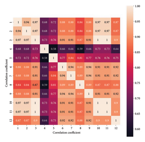
Eleven different states (normal, oil leakage, plugged holes, worn needle valve coupling bushings, reduced starting valve pressure, exhaust valve leakage, air cooler failure, turbocharger failure, lagged opening of intake valves, worn piston rings, and lagged injection advance angle) of 12 thermodynamic parameters were obtained through simulation with the AVL Boost model. The types and label information of the thermodynamic parameters are shown in Table 5. KNN-MI was used to select thermodynamic parameters with low correlation for fault diagnosis. The correlation matrix of thermodynamic parameters calculated using KNN-MI is shown in Figure 7, where a correlation coefficient greater than 0.9 is considered strongly correlated. After comprehensive evaluation, four thermodynamic parameters were finally selected, which correspond to the scavenge air box inlet pressure, scavenge air box inlet temperature, exhaust temperature, and indicated mean effective pressure.

Table 5. Thermodynamic parameter label information.

Fault type	Label
Compressor inlet pressure	1
Compressor inlet temperature	2
Compressor mass flow rate	3
Scavenge air box inlet pressure	4
Scavenge air box inlet temperature	5
Pressure at intake valve closure	6
Cylinder maximum explosion pressure	7
Exhaust temperature	8
Pressure at exhaust valve opening	9
Turbine inlet pressure	10
Turbine inlet temperature	11
Indicates the average effective pressure	12

4. Selection of Feature Parameter Fusion and Dimensionality Reduction Methods

Feature fusion and dimensionality reduction methods are used to integrate the 8 time-domain features and 12 frequency-domain features of the combustion segment vibration data with the selected thermodynamic parameters. The formula is shown in Table 6. Feature dimensionality reduction algorithms are an important technique in the field of machine learning, with the goal of mapping data from high-dimensional spaces to lower-dimensional spaces to facilitate data visualization, feature selection, and model training.

Table 6. Time-frequency domain equations.

Formula name	Equation
Peak-to-peak ratio	p₁ = max(x(n)) − min(x(n))
Average	$p_{2} = (\sum_{n = 1}^{N} x (n) / N)$
Variance	$p_{3} = (\sum_{n = 1}^{N} {(x (n) - p_{2})}^{2} / N - 1)$
Standard deviation	$p_{4} = \sqrt{(\sum_{n = 1}^{N} {(x (n) - p_{2})}^{2} / N - 1)}$
Root mean square value	$p_{5} = \sqrt{(\sum_{n = 1}^{N} {(x (n))}^{2} / N)}$
Square root amplitude	$p_{6} = (\sum_{n = 1}^{N} \sqrt{\|x (n)\|} / N)$
Skewness	$p_{7} = (\sum_{n = 1}^{N} {(x (n) - p_{2})}^{3} / (N - 1) p_{4}^{3})$
Steepness	$p_{8} = (\sum_{n = 1}^{N} {(x (n) - p_{2})}^{4} / (N - 1) p_{4}^{4})$
Waveform factor	p₉ = (max\|x(n)\|/p₅)
Crest factor	p₁₀ = (p₅/\|p₂\|)
Impulse factor	p₁₁ = (max\|x(n)\|/\|p₂\|)
Margin factor	p₁₂ = (max\|x(n)\|/p₆)
Frequency domain average	$p_{13} = (\sum_{k = 1}^{K} s (k) / K)$
Degree of spectrum concentration	$p_{14} = (\sum_{k = 1}^{K} {(s (k) - p_{13})}^{2} / K - 1)$ $p_{15} = (\sum_{k = 1}^{K} {(s (k) - p_{13})}^{3} / K {(\sqrt{p_{14}})}^{3})$ $p_{16} = (\sum_{k = 1}^{K} {(s (k) - p_{13})}^{4} / K p_{14}^{2})$
Center of gravity frequency	$p_{17} = (\sum_{k = 1}^{K} f_{k} s (k) / \sum_{k = 1}^{K} s (k))$
Master band position	$p_{18} = \sqrt{(\sum_{k = 1}^{K} f_{k}^{2} s (k) / \sum_{k = 1}^{K} s (k))}$ $p_{19} = \sqrt{(\sum_{k = 1}^{K} f_{k}^{4} s (k) / \sum_{k = 1}^{K} f_{k}^{2} s (k))}$ $p_{20} = (\sum_{k = 1}^{K} f_{k}^{2} s (k) / \sqrt{\sum_{k = 1}^{K} s (k) \sum_{k = 1}^{K} f_{k}^{4} s (k)})$

4.1. Linear Dimensionality Reduction

Feature dimensionality reduction algorithms can be divided into linear and nonlinear methods. Linear dimensionality reduction algorithms assume that the data in the original feature space follow a linear distribution, thus allowing the use of linear transformations to map the data into a lower-dimensional space. Common linear dimensionality reduction algorithms include PCA, independent component analysis (ICA), and linear discriminant analysis (LDA) [19]. Among them, LDA is a commonly used supervised learning algorithm, mainly applied in areas such as text classification, image classification, and bioinformatics. This paper’s data are not suitable for this method. Nonlinear dimensionality reduction algorithms assume that the data in the original feature space follow a nonlinear distribution, thus requiring the use of nonlinear transformations to map the data into a lower-dimensional space. Nonlinear dimensionality reduction algorithms can be divided into two categories: one is kernel-based algorithms, such as kernel principal component analysis (KPCA) and kernel independent component analysis (KICA). Since KICA is mainly used to deal with nonlinear relationships and independence in high-dimensional data, this paper does not provide further introduction to KICA. Another category of nonlinear dimensionality reduction algorithms is manifold learning dimensionality reduction algorithms, such as t-distributed stochastic neighbor embedding (t-SNE) and uniform manifold approximation and projection (UMAP) [20]. t-SNE uses the t-distribution stochastic neighbor embedding method to learn the manifold structure of the data and then maps it into a lower-dimensional space. Due to the disadvantage of the UMAP method that requires the selection of appropriate parameters and the parameters affect the results of the algorithm, this paper does not use this method for dimensionality reduction.

t-SNE is a nonlinear dimensionality reduction technique used for high-dimensional data visualization, especially suitable for embedding high-dimensional datasets into two-dimensional or three-dimensional spaces [21]. The following are some key mathematical concepts and formulas of t-SNE:

1.
Probability distribution in high-dimensional space: In the original high-dimensional space, the probability distribution of each point x_i is defined by a Gaussian (normal) distribution:
$\begin{matrix} P (x_{i}) = \frac{1}{\sqrt{2 π σ_{i}^{2}}} e^{- ({‖x_{i}‖}^{2} / 2 σ_{i}^{2})} . \end{matrix}$ ()
In the formula, σ_i is the scale parameter associated with point x_i.
2.
Probability distribution in low-dimensional space: In the embedded low-dimensional space (usually two-dimensional or three-dimensional), the probability distribution of each point y_i is defined by the t-distribution:
$\begin{matrix} P (y_{i}) = \frac{(1 + {‖y_{i}‖}^{2}) / (2 α)}{\sum_{j \neq i} (1 + {‖y_{i} - y_{j}‖}^{2}) / (2 α)} . \end{matrix}$ ()
In the formula, α is the shape parameter of the t-distribution.
3.
Calculation of similarity: The similarity between point pairs in the high-dimensional and low-dimensional spaces is usually calculated using the Gaussian kernel function:
$\begin{matrix} P_{i j}^{X} = \frac{e^{- ({‖x_{i} - x_{j}‖}^{2} / 2 σ_{i}^{2})}}{\sum_{k \neq l} e^{- ({‖x_{k} - x_{l}‖}^{2} / 2 σ_{i}^{2})}}, \\ P_{i j}^{Y} = \frac{e^{- {‖y_{i} - y_{j}‖}^{2} / 2 α}}{\sum_{k \neq l} e^{- {‖y_{k} - y_{l}‖}^{2} / 2 α}} . \end{matrix}$ ()
4.
t-SNE objective function: The goal of t-SNE is to minimize the Kullback–Leibler divergence between the similarity distributions in the high-dimensional and low-dimensional spaces:
$\begin{matrix} C = \sum_{i, j} P_{i j}^{X} \log \frac{P_{i j}^{X}}{P_{i j}^{Y}} . \end{matrix}$ ()
5.
Gradient calculation: To minimize the objective function C, it is necessary to compute the gradient with respect to the positions of the points in the low-dimensional space and use gradient descent or other optimization algorithms for optimization:
$\begin{matrix} \frac{\partial C}{\partial y_{i}} = 2 \sum_{j \neq i} (P_{i j}^{Y} - P_{i j}^{X}) (\frac{y_{i} - y_{j}}{1 + {‖y_{i} - y_{j}‖}^{2}} - \frac{α \cdot y_{i}}{1 + α^{2} {‖y_{i}‖}^{2}}) . \end{matrix}$ ()

The optimization process of t-SNE is typically divided into two stages: an early stage where a larger α value is used for compression to preserve the local structure of the high-dimensional space; and a late stage where a smaller α value is used for attraction to optimize the global layout. t-SNE often uses stochastic gradient descent to optimize the objective function, which is an iterative method that updates the embedding using only a random sample or a small batch of samples from the dataset at each iteration. t-SNE is a powerful tool, especially suitable for visualizing complex high-dimensional datasets, such as images, text, and gene expression data.

4.2. Comparison of Dimensionality Reduction Effects

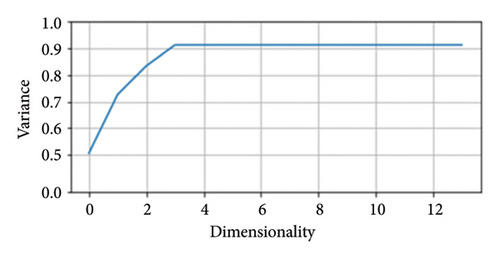
Twenty time-domain and frequency-domain features of vibration data are fused and reduced in dimension with four features extracted from thermodynamic parameters using the KNN-MI method. During the process of reducing the feature dimension, computational efficiency is improved, but some information is lost. Therefore, different dimensions of feature parameters retain different amounts of information in the data. To avoid the impact of the number of different dimensions retained on the four dimensionality reduction methods, a unified feature fusion and dimension reduction number is first determined using the PCA method.

Figure 8 shows the sum of variances when retaining different numbers of dimensions using the PCA method. The horizontal axis represents the number of dimensions retained, and the vertical axis represents the sum of variances of all components after dimensionality reduction. From the figure, we can observe that as the number of dimensions reduced increases, the proportion of the sum of variances first grows rapidly and then grows steadily. When the number of dimensions after reduction is 3, the sum of variances of all components is 90%, which means that 10% of the information is lost during the dimensionality reduction process. To ensure the information contained in the data after dimensionality reduction and to observe the data after reduction, the number of dimensions for feature fusion and dimensionality reduction is set to 3.

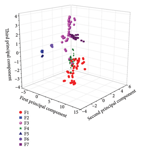
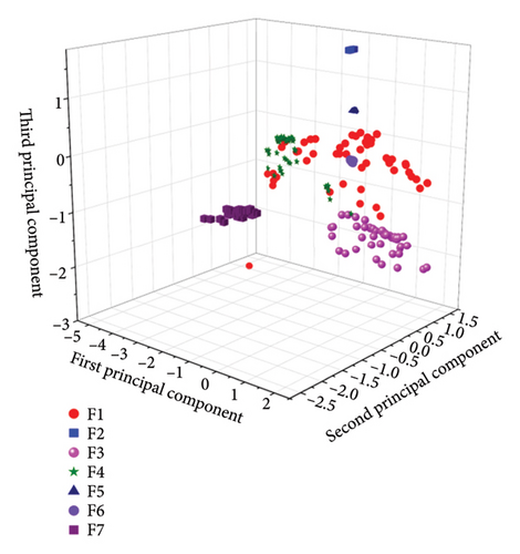
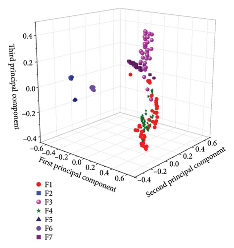
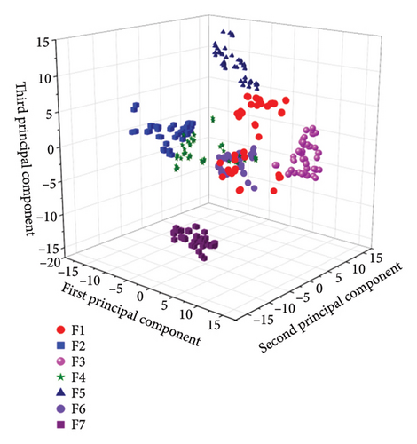
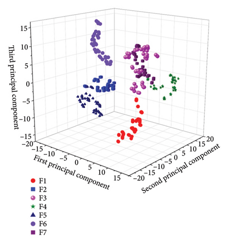
After determining the number of dimensions to reduce, the effects of the four dimensionality reduction methods are compared. Figure 9 shows the three-dimensional renderings after dimensionality reduction using the four methods, and Table 7 is a comparison table of fault information corresponding to different components based on data labels.

Table 7. Data label and fault correlation table.

Data label	Fault type	Sample quantity
F1	Nozzle clogging	50
F2	Wear of the nozzle needle valve	50
F3	Reduced pressure of the nozzle	50
F4	Normal	50
F5	Exhaust valve leakage	50
F6	Piston ring wear	50
F7	Single cylinder misfire	50

From Figure 9, it can be observed that after dimensionality reduction by the PCA algorithm, the interclass distances for the data types F1, F3, and F4 are small, while the intraclass distances are large. There is an overlap phenomenon among these three states’ data, and due to severe congestion, it is difficult to implement classification, resulting in average classification effects. After dimensionality reduction by the ICA algorithm, the interclass distances for the data types F1, F3, and F4 are small, with an overlap phenomenon, and these three fault states cannot be completely and effectively separated, resulting in average classification effects. After dimensionality reduction by the KPCA algorithm, except for the large intraclass distances of F1 and F4, the intraclass distances of other data types are small, and the interclass distances are large, leading to good classification effects. After dimensionality reduction by the t-SNE algorithm, the characteristics shown are small intraclass distances and large interclass distances, with no obvious overlap phenomena between different types of data, resulting in good classification effects. After comprehensively comparing the effects of the four dimensionality reduction methods, the t-SNE algorithm is ultimately selected as the feature parameter fusion and dimensionality reduction method.

5. Diesel Engine Fault Diagnosis Model Based on Feature Parameter Fusion

Using the t-SNE dimensionality reduction method, the time-domain and frequency-domain features of the cylinder head vibration are fused with the thermodynamic parameters selected by KNN-MI to construct a feature fusion dataset. SVM is used for data classification and recognition, constructing a diesel engine fault diagnosis model based on feature parameter fusion to distinguish the types of faults occurring.

5.1. Analysis of Feature Fusion Effectiveness

To prove the effectiveness of feature fusion, a comparative analysis is made between the dimensionality reduction effects of single vibration signal features and multifeature fusion. Figure 10 shows the comparison effect of a single vibration signal feature after t-SNE dimensionality reduction. From the figure, it can be seen that the characteristics of this single signal source feature after dimensionality reduction are large intraclass distances, large interclass distances, and obvious overlap phenomena between different types of data, resulting in poor classification effects. In contrast, after feature fusion and dimensionality reduction, the same type of data is in the same area, with a higher concentration and small intraclass distances. Different types of data are distributed in different positions, and the boundaries between data are clear. Large interclass distances and high discrimination can better distinguish different types of diesel engine faults.

5.2. Fault Diagnosis Model

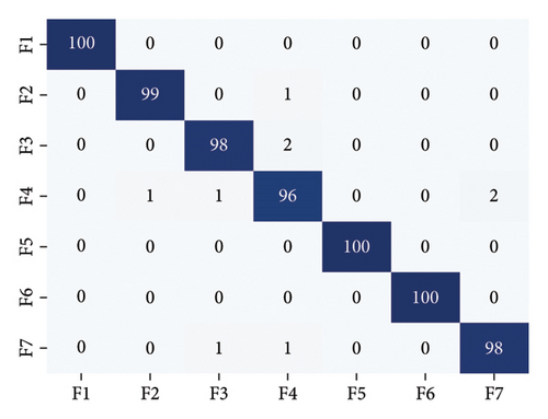
To eliminate errors caused by visual observation, only the recognition accuracy of the single vibration signal features and the four feature fusion dimensionality reduction methods will be compared. A unified SVM classifier is used to classify the dataset, with a training set to test set ratio of 2 : 1 (segmentation of test and training sets based on the size of the categorical data, the complexity of the model, and the objectives of the task). Table 8 provides the dataset information. Table 9 shows the recognition accuracy of different component data types. Figure 11 shows the confusion matrix of recognition accuracy after dimensionality reduction by t-SNE feature fusion, and Table 10 shows the TPR, FPR, and TNR values of the changed confusion matrix.

Table 8. Dataset information.

Data label	Fault type	Sample quantity
F1	Nozzle clogging	300
F2	Wear of the nozzle needle valve	300
F3	Reduced pressure at nozzle opening	300
F4	Normal	300
F5	Exhaust valve leakage	300
F6	Piston ring wear	300
F7	Single cylinder misfire	300

Table 9. Recognition accuracy for different data types.

Data type	Diagnostic accuracy (%)
Single vibration signal feature dimensionality reduction	78.8
Vibration and thermodynamic parameters fused with PCA dimensionality reduction	96.2
Vibration and thermodynamic parameters fused with ICA dimensionality reduction	94.1
Vibration and thermodynamic parameters fused with KPCA dimensionality reduction	96.4
Vibration and thermodynamic parameters fused with t-SNE dimensionality reduction	98.7

Table 10. TPR, FPR, and TNR for Figure 11.

Data type	TPR	FPR	TNR
F1	1.0000	0.0000	1.0000
F2	0.9900	0.0017	0.9983
F3	0.9800	0.0033	0.9967
F4	0.9600	0.0067	0.9933
F5	1.0000	0.0000	1.0000
F6	1.0000	0.0000	1.0000
F7	0.9800	0.0033	0.9967

From Table 9, it can be observed that the recognition accuracy using feature fusion dimensionality reduction methods is higher than that of single vibration signal feature dimensionality reduction, which proves that using a multisource information fusion approach to integrate cylinder head vibration with thermodynamic parameters through dimensionality reduction can effectively distinguish the types of diesel engine faults. Additionally, the recognition accuracy after fusion and dimensionality reduction of vibration and thermodynamic parameters using t-SNE is the highest, proving that the dimensionality reduction effect of the t-SNE method is good, demonstrating the superiority of this dimensionality reduction method. From Figure 8 and Table 10, it can be seen that the overall classification is good, in which F4 samples were misclassified as F2/F3/F7 in total 4 cases, while the samples of other classes were misclassified as F4 in total 4 cases, which indicates that the fault may be confounded with features of other classes.

6. Conclusions

In response to the issue that different components of a diesel engine may exhibit the same fault phenomenon, that is, one effect with multiple causes, and the complex and diverse causes of faults leading to a low identification rate of fault diagnosis methods, a diesel engine typical fault diagnosis method using multisource information fusion was adopted. Using t-SNE to integrate multiple time-domain and frequency-domain features of cylinder head vibration with thermodynamic parameters selected by the KNN-MI method, a feature parameter fusion dataset was constructed, and SVM was used for data classification and recognition, effectively identifying various faults of the diesel engine. This provides a solution to the problem of the low identification rate of fault diagnosis methods caused by the complexity and diversity of diesel engine fault causes, one effect with multiple causes. The following conclusions are mainly drawn:

1.
Based on the AVL Boost platform, a simulation model of the target machine was built, and the model was calibrated and validated with experimental data. The error between the simulation results and the experimental results is within 3%, and the model can simulate the changes of thermodynamic parameters of the diesel engine under different states, providing thermodynamic parameters for multisource information fusion diagnosis methods.
2.
The KNN-MI was used to select thermodynamic parameters, eliminating those with strong correlations, and ultimately four thermodynamic parameters with low correlations were selected for fusion with vibration feature parameters.
3.
A comprehensive comparison of the dimensionality reduction effects of four different methods when fusing vibration feature parameters with selected thermodynamic parameters showed that the t-SNE dimensionality reduction method resulted in small intraclass distances for the same type of fault samples and large interclass distances for different types of fault samples, effectively distinguishing various types of diesel engine faults.
4.
The classification and identification accuracy of only a single vibration signal is only 78.8%, which is due to the fact that the faults of different parts of the diesel engine may show the same fault phenomenon, resulting in a low fault identification rate. In the article, the recognition accuracy is increased to 98.7% by fusing the thermal parameters and vibration data for dimensionality reduction, which proves that the use of the multisource information fusion method to fuse the cylinder head vibration with the thermal parameters for dimensionality reduction can effectively differentiate the types of diesel engine faults.

In the later research work, we apply the method to different diesel engine models to explore the practical utility of the scheme and use multiple classification methods for identification to further improve the accuracy of fault diagnosis. In addition, in diesel engine fault diagnosis, dynamic changes in operating conditions, such as fluctuations in rotational speed and load, affect the characteristics of the vibration signals, which in turn change the distribution of the data in the feature space, resulting in inconsistent distributions of the training and test data and affecting the generalization performance of the data-driven fault diagnosis method, which will be migrated to achieve cross-conditional fault diagnosis of diesel engines.

Conflicts of Interest

The authors declare no conflicts of interest.

Funding

This work was supported by the National Natural Science Foundation of China (grant no. 52271328).

Acknowledgments

This work was supported by the National Natural Science Foundation of China (grant no. 52271328).

Open Research

Data Availability Statement

The data used to support the findings of this study are included within the article.

References

1 Yan G., Hu Y., and Jiang J., A Novel Fault Diagnosis Method for Marine Blower With Vibration Signals, Polish Maritime Research. (2022) 29, no. 2, 77–86, https://doi.org/10.2478/pomr-2022-0019.
10.2478/pomr-2022-0019
Google Scholar
2 Li C., Chen C., and Gu X., Acoustic Signal Analysis for Gear Fault Diagnosis Using a Uniform Circular Microphone Array, Journal of Mechanical Science and Technology. (2023) 37, no. 11, 5583–5596, https://doi.org/10.1007/s12206-023-1002-8.
10.1007/s12206-023-1002-8
Google Scholar
3 Matulić N., Radica G., and Nižetić S., Engine Model for Onboard Marine Engine Failure Simulation, Journal of Thermal Analysis and Calorimetry. (2020) 141, no. 1, 119–130, https://doi.org/10.1007/s10973-019-09118-3.
10.1007/s10973-019-09118-3
CAS Google Scholar
4 Safizadeh M. S. and Latifi S. K., Using Multi-Sensor Data Fusion for Vibration Fault Diagnosis of Rolling Element Bearings by Accelerometer and Load Cell, Information Fusion. (2014) 18, 1–8, https://doi.org/10.1016/j.inffus.2013.10.002, 2-s2.0-84887493381.
10.1016/j.inffus.2013.10.002
Web of Science® Google Scholar
5 Nacchia M., Fruggiero F., Lambiase A. et al., A Systematic Mapping of the Advancing Use of Machine Learning Techniques for Predictive Maintenance in the Manufacturing Sector, Applied Sciences. (2021) 11, no. 6, https://doi.org/10.3390/app11062546.
10.3390/app11062546
Google Scholar
6 Montero Jimenez J. J., Schwartz S., Vingerhoeds R., Grabot B., and Salaün M., Towards Multi-Model Approaches to Predictive Maintenance: A Systematic Literature Survey on Diagnostics and Prognostics, Journal of Manufacturing Systems. (2020) 56, 539–557, https://doi.org/10.1016/j.jmsy.2020.07.008.
10.1016/j.jmsy.2020.07.008
Google Scholar
7 Gawde S., Patil S., Kumar S., Kamat P., Kotecha K., and Abraham A., Multi-Fault Diagnosis of Industrial Rotating Machines Using Data-Driven Approach: A Review of Two Decades of Research, Engineering Applications of Artificial Intelligence. (2023) 123, https://doi.org/10.1016/j.engappai.2023.106139.
10.1016/j.engappai.2023.106139
Google Scholar
8 Huang M. and Liu Z., Research on Mechanical Fault Prediction Method Based on Multifeature Fusion of Vibration Sensing Data, Sensors. (2019) 20, no. 1, https://doi.org/10.3390/s20010006.
10.3390/s20010006
Web of Science® Google Scholar
9 Huang X., Wu L., and Ye Y., A Review on Dimensionality Reduction Techniques, International Journal of Pattern Recognition and Artificial Intelligence. (2019) 33, no. 10, https://doi.org/10.1142/s0218001419500174, 2-s2.0-85062616939.
10.1142/S0218001419500174
Google Scholar
10 Meng T., Jing X., Yan Z., and Pedrycz W., A Survey on Machine Learning for Data Fusion, Information Fusion. (2020) 57, 115–129, https://doi.org/10.1016/j.inffus.2019.12.001.
10.1016/j.inffus.2019.12.001
Web of Science® Google Scholar
11 Kong L., Peng X., Chen Y., Wang P., and Xu M., Multi-Sensor Measurement and Data Fusion Technology for Manufacturing Process Monitoring: A Literature Review, International Journal of Extreme Manufacturing. (2020) 2, no. 2, https://doi.org/10.1088/2631-7990/ab7ae6.
10.1088/2631-7990/ab7ae6
Google Scholar
12 Guan H., Ren Y., Tang H., and Xiang J., Intelligent Fault Diagnosis Methods for Hydraulic Components Based on Information Fusion: Review and Prospects, Measurement Science and Technology. (2024) 35, no. 8, https://doi.org/10.1088/1361-6501/ad437e.
10.1088/1361-6501/ad437e
PubMed Google Scholar
13 Liu G., Zhou X., Xu X., Wang L., and Zhang W., Fault Diagnosis of Diesel Engine Information Fusion Based on Adaptive Dynamic Weighted Hybrid Distance-Taguchi Method (ADWHD-T), Applied Intelligence. (2022) 52, no. 9, 10307–10329, https://doi.org/10.1007/s10489-021-02962-7.
10.1007/s10489-021-02962-7
Google Scholar
14 Qian L., Li B., and Chen L., CNN-Based Feature Fusion Motor Fault Diagnosis, Electronics. (2022) 11, no. 17, https://doi.org/10.3390/electronics11172746.
10.3390/electronics11172746
Google Scholar
15 Elsamanty M., Ibrahim A., and Salman W. S., Principal Component Analysis Approach for Detecting Faults in Rotary Machines Based on Vibrational and Electrical Fused Data, Mechanical Systems and Signal Processing. (2023) 200, https://doi.org/10.1016/j.ymssp.2023.110559.
10.1016/j.ymssp.2023.110559
Google Scholar
16 Fu Y., Liu Y., and Gao Z., Fault Classification in Wind Turbines Using Principal Component Analysis Technique, 1, Proceedings of the 2019 IEEE 17th International Conference on Industrial Informatics (INDIN), July 22–25, 2019, Helsinki, Finland, IEEE, 1303–1308, https://doi.org/10.1109/indin41052.2019.8972303.
10.1109/indin41052.2019.8972303
Google Scholar
17 Lei Y., Jiang W., Jiang A., Zhu Y., Niu H., and Zhang S., Fault Diagnosis Method for Hydraulic Directional Valves Integrating PCA and XGBoost, Processes. (2019) 7, no. 9, https://doi.org/10.3390/pr7090589, 2-s2.0-85072155069.
10.3390/pr7090589
Web of Science® Google Scholar
18 Woschni G., A Universally Applicable Equation for the Instantaneous Heat Transfer Coefficient in the Internal Combustion Engine. No. 670931, SAE Technical Paper Series. (1967) https://doi.org/10.4271/670931, 2-s2.0-1842565645.
10.4271/670931
Google Scholar
19 Zhu X., Wang Y., Li Y., Tan Y., Wang G., and Song Q., A New Unsupervised Feature Selection Algorithm Using Similarity-Based Feature Clustering, Computational Intelligence. (2019) 35, no. 1, 2–22, https://doi.org/10.1111/coin.12192, 2-s2.0-85054381782.
10.1111/coin.12192
Web of Science® Google Scholar
20 Anowar F., Sadaoui S., and Selim B., Conceptual and Empirical Comparison of Dimensionality Reduction Algorithms (PCA, KPCA, LDA, MDS, SVD, LLE, ISOMAP, LE, ICA, T-SNE), Computer Science Review. (2021) 40, https://doi.org/10.1016/j.cosrev.2021.100378.
10.1016/j.cosrev.2021.100378
Google Scholar
21 Belkina A. C., Ciccolella C. O., Anno R., Halpert R., Spidlen J., and Snyder-Cappione J. E., Automated Optimized Parameters for T-Distributed Stochastic Neighbor Embedding Improve Visualization and Analysis of Large Datasets, Nature Communications. (2019) 10, no. 1, https://doi.org/10.1038/s41467-019-13055-y.
10.1038/s41467-019-13055-y
PubMed Google Scholar

All articles

A Fault Diagnosis Method for Typical Failures of Marine Diesel Engines Based on Multisource Information Fusion

Abstract

1. Introduction

2. Acquisition and Analysis of Cylinder Head Vibration Signals for Typical Diesel Engine Faults