Automatic Identification of Diverse Tunnel Threats With Machine Learning–Based Distributed Acoustic Sensing
Abstract
As the backbone of modern urban underground traffic space, tunnels are increasingly threatened by natural disasters and anthropogenic activities. Current tunnel surveillance systems often rely on labor-intensive surveys or techniques that only target specific tunnel events. Here, we present an automated tunnel monitoring system that integrates distributed acoustic sensing (DAS) technology with ensemble learning. We develop a fiber-optic vibroacoustic dataset of tunnel disturbance events and embed vibroscape data into a common feature space capable of describing diverse tunnel threats. On the scale of seconds, our anomaly detection pipeline and data-driven stacking ensemble learning model enable automatically identifying nine types of anomalous events with high accuracy. The efficacy of this intelligent monitoring system is demonstrated through its application in a real-world tunnel, where it successfully detected a low-energy but dangerous water leakage event. The highly generalizable machine learning model, combined with a universal feature set and advanced sensing technology, offers a promising solution for the autonomous monitoring of tunnels and other underground spaces.
1. Introduction
Underground infrastructure constitutes the backbone of the economic life of modern cities [1]. Tunnels are important underground transportation spaces [2]. With the development of ultra-deep and ultra-long tunnels, and due to the complexity of geologic conditions and various anthropogenic activities, tunnels are increasingly threatened by a range of disasters such as groundwater inflows, rock bursts, rockfalls, and tunnel breakdown [3, 4], during both construction and operation. Therefore, ensuring the secure construction and operation of tunnels, as well as the timely anticipation of impending risks, requires diligent monitoring and assessment of the safety and stability status of the tunnels.
On-site monitoring for tunnel safety is broadly divided into contact and noncontact techniques [5]. Contact methods utilize physical point sensors attached to the tunnel structure to evaluate stability and safety [6]. For example, microseismic monitoring employs seismic sensors to detect microseismic activities in the surrounding rock mass, providing early warnings of tunnel rockburst disasters [7]. Strain gauges measure strain changes within tunnel structures, highlighting potential issues such as stress concentrations or cracks [8]. Temperature sensors identify leakage events by monitoring temperature variations of tunnel lining segments [9]. However, these point-based methods can fail to detect localized issues that develop between sensor placements, potentially leading to unnoticed structural weaknesses [10]. Furthermore, once installed, contact sensors are stationary and cannot be easily relocated, limiting their adaptability to evolving tunnel conditions. Contactless methods include vision-based methods (e.g., digital photogrammetry [11], robot inspections [12]), acoustic techniques [13], three-dimensional laser scanning [14], and infrared thermographic monitoring [15]. Despite providing high-precision data, noncontact methods face challenges such as high equipment costs, complex data processing requirements, and susceptibility to rapidly changing environmental conditions within tunnels. For example, vision-based and laser-based techniques can be compromised by dust, water vapor, or other particulate matter, which scatter or absorb signals, thereby degrading data quality and complicating the differentiation of true structural changes from noise [12]. While traditional tunnel monitoring methods, including threshold-based detection, frequency-domain analysis, and statistical models, have been widely used, they often require manual tuning and rely on predefined parameters, making them sensitive to noise and environmental variability. These methods typically extract single features, which may not fully capture the complexity of distributed acoustic sensing (DAS) signals. Despite significant advancements, no current method achieves the desired level of real-time monitoring and spatial resolution necessary for comprehensive and diverse threat identification in tunnel environments.
Recently, DAS—a fiber-optic sensing technology that allows for dense large-aperture vibroacoustic measurements [16, 17]—has emerged rapidly as a powerful tool for perimeter security surveillance, oil and gas well diagnosis, and seismic observation and imaging [18–21]. Based on the principle of phase-sensitive optical time-domain reflectometry (ϕ-OTDR), DAS can perform array measurements of vibrations over tens of kilometers of common fiber-optic cable with high sensitivity and reliability, potentially enabling time-lapse monitoring of tunnel safety by characterizing its “vibroscape”—a term used to describe the overall characteristics of environmental vibration signals [22]. This approach integrates various disturbance events into a unified feature space, allowing for comprehensive threat analysis. DAS has excellent reliability and anti-interference performance. By incorporating specially designed sheaths, the optical fibers can operate in diverse environmental conditions, including high temperatures, high humidity, and high pressure, making DAS well suited for complex tunnel environments.
A striking feature of DAS-based vibroacoustic monitoring is that the sensing fiber array is interrogated at a channel spacing of the order of decimeters, leading to data volumes that are tens to hundreds of times larger than the traditional point-wise microseismic monitoring. For example, a field experiment on a 20-km dark fiber cable (sampled at 500 Hz) has collected about 12 terabytes of data over a period of 40 days [23]. Such acquisition fashions and datasets challenge current models of data storage, transmission, and analysis, thus hindering real-time monitoring and immediate decision-making. Therefore, it is an urgent task to develop a common framework that can efficiently handle huge volumes of DAS data, especially to automatically detect and rapidly identify anomalies in noisy environments.
An appealing strategy for DAS data processing and event recognition is to use machine learning [24]. Yet to date, most machine learning–based DAS studies reported have used only one algorithm (e.g., support vector machine [SVM], eXtreme gradient boosting [XGBoost], and random forest [RF]) for classification [25–27], and comparative studies have mostly employed a reduced set of fiber-optic vibrational events (mostly three-class classification problems) that cover limited ground and geographical conditions [28, 29]. There is no conclusive answer as to which machine learning algorithm has the best predictive performance for DAS-recorded engineering vibroacoustic signals. Importantly, so far, there are a very few reported research efforts [30] that are dedicated to tunnel condition monitoring. Models built for other scenarios may not be directly applicable to tunnel environments, as there can be significant differences in the best machine learning strategy and the most predictive feature set.
This study includes the following three contributions: (1) we proposed a novel integrated framework for automated tunnel threat monitoring using machine learning and DAS-recorded vibroscapes. Our approach also includes an effective anomaly detection pipeline including signal picking, separation, and filtering to extract vibration signals from random background noise. (2) We developed a publicly available DAS dataset of tunnel vibrational events. We selected highly predictive features of vibration signals to describe diverse tunnel threats, focusing on time- and frequency-domain properties. (3) We performed DAS measurements of vibrational events in the Beijing–Xiong’an (Jing–Xiong) intercity railway tunnel (Hebei, China) to validate the proposed approach. Our system successfully identified events such as leakage, excavation activities, and vehicle passage with high accuracy.
The remainder of this paper is organized as follows. Section 2 details the architecture of the proposed ML-based DAS monitoring system. Section 3 describes the methods used for dataset acquisition from real tunnels. Section 4 presents the outcomes of training and evaluation, including the impact of key factors. Section 5 showcases the application of our system in the Jing–Xiong intercity railway tunnel. Section 6 provides a summary of this paper and discusses future directions for using DAS in tunnel safety monitoring.
2. Methodology
2.1. Overview
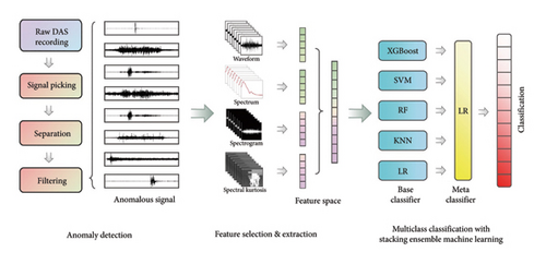
As illustrated in Figure 1, we present a novel framework for the automated monitoring of tunnel disturbance events using machine learning and DAS-recorded vibroscapes. The framework consists of three subsystems: anomaly detection, feature selection, and multiclass recognition. In the anomaly detection subsystem, we utilize the improved STA/LTA method along with the normalized cumulative energy curve to swiftly and accurately identify tunnel vibration events from extensive real-time DAS background noise. Subsequently, the signal denoising algorithm is employed to denoise the vibration signals, enhancing the signal-to-noise ratio (SNR). Regarding feature selection, the elastic net algorithm is employed to circumvent collinearity and reduce the dimensionality of the feature space, thereby selecting high-quality features for subsequent classification. The third subsystem is a machine learning–based automatic classification module. We employ a stacking ensemble learning strategy to train and optimize a combination of well-performing classification algorithms with our feature set through cross-validation [31].
2.2. Automated Anomaly Detection
2.2.1. Self-Adjusted Signal Picking and Separation Procedures
The duration of the detected signal can be measured by dual-thresholding in the STA/LTA algorithm. The low threshold sensitively captures the energy change of the time series and preliminarily obtains the initiation point of the signal. However, there are two cases that can trigger a low threshold including the onset of the signal and accidental high-energy noise, making further classification via high thresholding necessary. The signal is considered to trigger on only when the STA/LTA ratio reaches the high threshold and lasts for at least 0.01 s. And if the STA/LTA ratio of this moment and the following five sliding windows are simultaneously less than the low threshold, the signal can be triggered off. Finally, we add 1 second of data before and after the duration to ensure the completeness of the signal. In addition, weather affects transportation [33] and topsoil conditions, which in turn biases the SNR of the same event. Therefore, the low threshold is dynamically adjusted to suppress the impact of environmental noise. Every hour, the system calculates a logarithmic root-mean-square (RMS) ratio of a 5-second background noise to the standard noise and integrates that ratio to the low threshold. A noisier environment produces a positive ratio, while a quieter environment produces a negative ratio; this enables dynamic fine-tuning of the base threshold. In this manner, false triggering on noisy signals can be minimized.
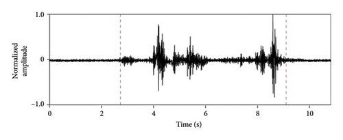
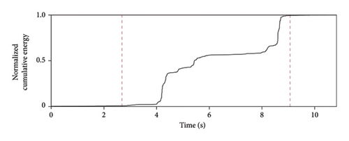
To extract the detected signals from the ambient vibration recordings while discarding unwanted data, we used the normalized cumulative energy curve [34], which allowed us to separate the signals of interest from the background noise in real time. Based on the interval extracted by STA/LTA, the trigger on/off of an event can be accurately computed by setting any two fractions of the normalized cumulative integral curve of the squared signal amplitude. In this work, we use 0.5% and 99.5% of the maximum to determine the start–stop points.
By combining these two algorithms, we can separate the detected signal from the background noise in real time. In this way, only signals of tunnel-disturbing events are left, while large, redundant DAS data are discarded.
2.2.2. Signal Denoising Methods
Our system next eliminates potential noise in the extracted signals, as their quantitative parameters can be biased by low SNRs. To achieve the best denoising performance, we evaluated four frequency-domain filters, namely, empirical mode decomposition (EMD), complementary ensemble empirical mode decomposition (CEEMD), variational mode decomposition (VMD), and wavelet threshold denoising (WTD). Among them, VMD and WTD are known as powerful denoisers with rich sets of adjustable parameters [35, 36], while EMD and CEEMD have relatively fewer parameters [37, 38] Time-domain filters that act essentially as data smoothers were not included in this comparison because they are very time-consuming and may ignore subtle variations in signal details. In addition, we did not consider band-pass filtering because it requires an a priori knowledge of the frequency attributes of signals and ignores time effects. Three metrics—SNR, root-mean-square error (RMSE), and smoothness—were used to quantitatively assess these methods. The parameter settings of the denoising algorithms are given in Table 1.
| Filter | Parameter | Explanation |
|---|---|---|
| CEEMD | Nstd = 0.5 | Ratio of the standard deviation of added white noise to the standard deviation of raw signal |
| NR = 50 | Number of iterations (number of noise additions) | |
| VMD | K = 5 | Mode number |
| Alpha = 2000 | Penalty coefficient | |
| Tol = 1e − 6 | Convergence tolerance | |
| WTD | db3 | Wavelet name |
| Soft threshold | Threshold function | |
| Lev = 4 | Decomposition level | |
| EMD | — | A function in MATLAB without adjusting parameters |
- Abbreviations: CEEMD, complementary ensemble empirical mode decomposition; EMD, empirical mode decomposition; VMD, variational mode decomposition; WTD, wavelet threshold denoising.
2.3. Elastic-Net Regression for Feature Selection
After signal denoising, the multithreat monitoring system automatically extracts signal features and then passes them to the machine learning–based pattern recognition subsystem. To construct a common, highly descriptive feature set for diverse tunnel vibration events, we examined a wide range of signal features [39]. We initially screened 11 waveform features, 4 spectral features, 5 spectrogram features, and 4 spectral kurtosis features, totaling 24 features (Table 2).
| Signal features | Abbreviation or acronym | |
|---|---|---|
| Waveform features | ||
| 1 | Mean | — |
| 2 | Peak-to-peak | P-P |
| 3 | Average rectified valuea | ARV |
| 4 | Variance | — |
| 5 | Kurtosisb | — |
| 6 | Skewnessc | — |
| 7 | Root mean square | RMS |
| 8 | Form factord | FF |
| 9 | Crest factore | CF |
| 10 | Impulse factorf | IF |
| 11 | Clearance factorg | CLF |
| Spectral features | ||
| 12 | Spectral centroid frequency | SCF |
| 13 | Mean square frequency | MSF |
| 14 | Variance of normalized power spectral density (PSD) | PSD.V |
| 15 | Standard deviation of normalized PSD | PSD.SD |
| Spectrogram featuresh | ||
| 16 | Area of binary image | Area |
| 17 | Perimeter of binary image | Perimeter |
| 18 | Compactness ratio of binary image | CR |
| 19 | Connected component of binary image | CC |
| 20 | Euler number of binary image | Eu |
| Spectral kurtosis features | ||
| 21 | Mean of spectral kurtosis | SK.Mean |
| 22 | Standard deviation of spectral kurtosis | SK.SD |
| 23 | Skewness of spectral kurtosis | SK.skewness |
| 24 | Kurtosis of spectral kurtosis | SK.kurtosis |
- aMean of the absolute value of the signal.
- bPeakness of the signal.
- cAsymmetry of a signal distribution.
- dRMS divided by the mean of the absolute value of the signal.
- ePeak value divided by the RMS of the signal.
- fThe height of a peak to the mean level of the signal.
- gPeak value divided by the squared mean value of the square roots of the absolute amplitudes of the signal.
- hFeatures of binary image by short-time Fourier transform.
To determine the optimal solution of α and λ, we employed the cross-validation technique. We first selected 100 groups of α values (between 0 and 1 with 0.01 increment) for a threefold cross-validation. Next, we performed another threefold cross-validation, which was repeated 10,000 times for different λ values.
2.4. Stacking Model for Multiclass Classification
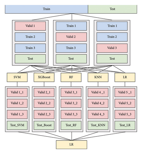
The last part of our system is built on an intelligent multithreat identification model that automatically distinguishes and classifies diverse tunnel disturbances by jointly analyzing the input multidimensional features. In an attempt to create a model with good recognition performance and generalization ability, we used stacking ensemble learning [42], which is a hybrid learning strategy where multiple machine learning models are optimally combined for obtaining better classification results than any single model in the ensemble. The architecture of a stacking ensemble learning model involves a diverse range of base models and a meta model that combines the predictions of the base models. Due to the nature of stacked ensembles, it typically yields better predictive performance than individual models. In this section, we will present the framework of stacking ensemble learning, including the design of base classifiers and the meta-classifier. Performance evaluation and comparisons with individual classifiers will be provided in Section 4.4.
Figure 2 illustrates the architecture of the stacking ensemble learning model. The stacking framework has a two-level structure: the first base-classifier layer and the second meta-classifier layer. We first split the data into a training set and a test set in a 7:3 ratio. After three pieces of training, the predictions of the entire original training set were obtained. This was repeated for each base classifier to form a new training set for the meta classifier. Next, we trained the base classifiers with the original training set to obtain predictions of the test set, which were used as a new test set. Finally, the meta classifier was trained using the new training set and tested with the new test set to generate final classifications. Since the training set of the meta classifier is not involved in the training of each base classifier, overfitting can be effectively avoided. In addition, the meta classifier integrates the outputs of the base classifiers, thus improving the overall accuracy of the model.
Base-classifier design is critical to stacking ensemble learning. We compared 10 classification algorithms that cover a variety of popular methods for machine learning algorithms: SVM, XGBoost, RF, logistic regression (LR), k-nearest neighbor (KNN), multilayer perceptron (MLP), Naive Bayes (NB), long short-term memory (LSTM), probabilistic neural network (PNN), and back-propagation (BP) neural network. In order to improve the classification performance of base classifiers, we employed particle swarm optimization (PSO) optimization techniques [43] to automatically tune the hyperparameters of the base models.
3. Data Preparation
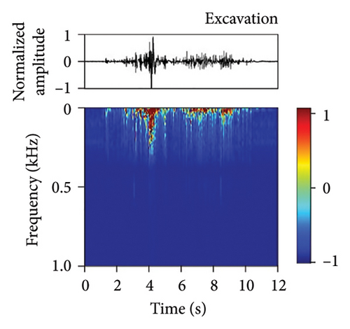
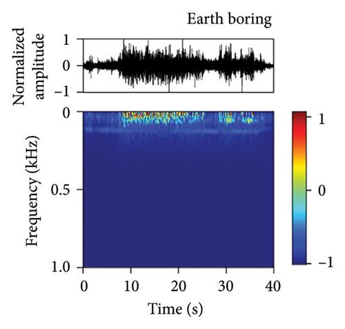
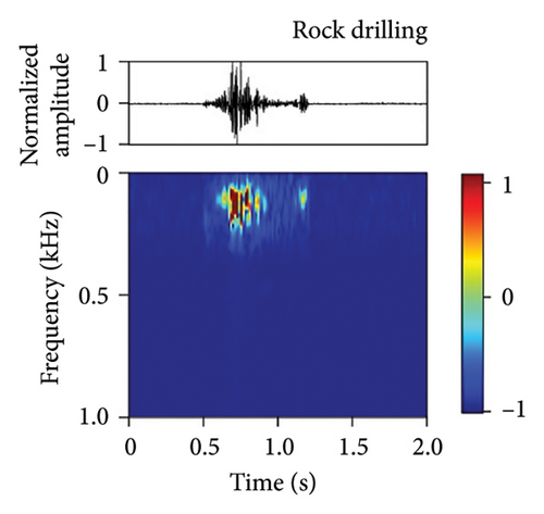
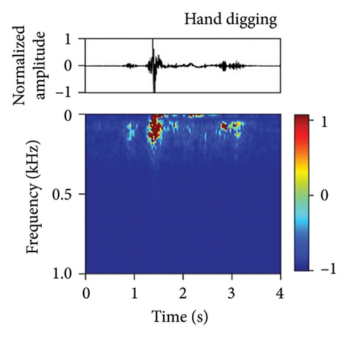
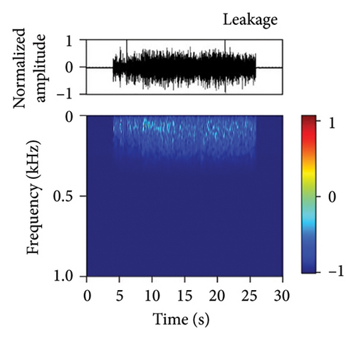
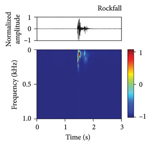
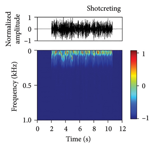
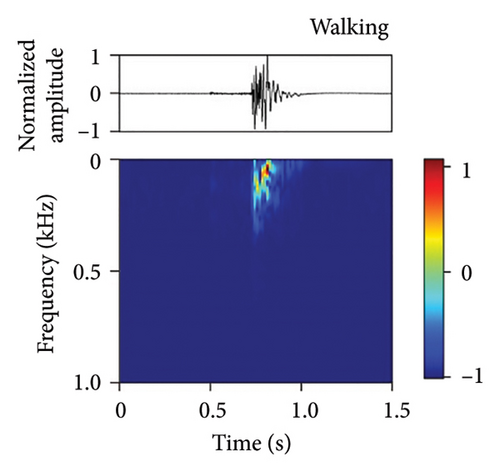
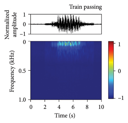
We have developed a fiber-optic DAS dataset of tunnel disturbance events. The dataset is composed of 1,494 signals from nine types of tunnel-threatening vibration events that cover both the tunnel construction and operation periods, including excavation (174), earth boring (139), rock drilling (265), hand digging (172), water leakage (32), rockfall (167), shotcreting (166), walking (276), and train passing (103) (the sample size in each type is given in parentheses). The data were collected from various tunnels that span tunnel types, soil conditions, and geographical conditions. To avoid an unbalanced dataset that may bias the performance of our trained model, we performed simulation experiments in a real tunnel environment to increase the sample size of the rockfall category (141 out of 167 samples are from the simulations). Example waveforms and spectrograms of the nine types of events are shown in Figure 3, together with a table summarizing their durations, frequency ranges, and waveform characteristics (Table 3).
| Event | Duration (s) | Frequency (Hz) | Waveform characteristics |
|---|---|---|---|
| Ambient noise | Random | Random | Continuous with random fluctuations, weak energy |
| Earth boring | 8.00–30.00 | 20–80 | Continuous and stable, strong energy |
| Excavation | 6.00–10.00 | 0–50 | Continuous but fluctuating, strong energy |
| Train passing | 5.00–6.00 | 0–120 | Continuous, strong energy |
| Hand digging | 4.00–6.00 | 50–200 | Continuous but fluctuating, weak energy |
| Rockfall | 0.40–0.80 | 0–350 | Abrupt jumping, strong energy, rapid decay |
| Walking | 0.06–0.09 | 0–160 | Abrupt jumping, weak energy |
| Rock drilling | 0.01–0.03 | 70–280 | Continuous and stable, strong energy |
| Water leakage | — | 80–350 | Continuous but fluctuating, weak energy |
| Shotcreting | — | 50–300 | Continuous and stable, strong energy |
Imbalanced datasets can affect the accuracy of machine learning models, biasing toward majority categories. Generally, if the sample sizes of different categories differ by a factor of 100 or more [44], standard performance measures may not be effective and would need modification. To evaluate the appropriateness of sample size distribution in our dataset, we performed a computational experiment as follows. First, we assumed that our dataset is unbalanced and solves the problem by using a resampling strategy. Specifically, we balanced the dataset by oversampling (or undersampling) to increase (respectively, decrease) the sample size in each category while keeping the total sample number constant (see Table 4 for the original and balanced distributions of event categories). Then, we trained three ML models on the original and resampled datasets by implementing a threefold cross-validation framework. The results show that dataset resampling had a very limited impact on the accuracy of the models, indicating that the sample size is appropriate for each type in our dataset (Table 5).
| Event category | Original | Resampled |
|---|---|---|
| Excavation | 174 | 166 |
| Earth boring | 139 | 166 |
| Rock drilling | 265 | 166 |
| Hand digging | 172 | 166 |
| Water leakage | 32 | 166 |
| Rockfall | 167 | 166 |
| Shotcreting | 166 | 166 |
| Walking | 276 | 166 |
| Train passing | 103 | 166 |
| Model | Metric | Score (original dataset) (%) | Score (balanced dataset) (%) |
|---|---|---|---|
| SVM | Accuracy | 96.44 | 96.65 |
| Precision | 96.70 | 96.68 | |
| Recall | 95.68 | 95.73 | |
| F1-score | 96.15 | 95.78 | |
| RF | Accuracy | 93.76 | 94.10 |
| Precision | 94.08 | 94.49 | |
| Recall | 93.48 | 93.67 | |
| F1-score | 93.70 | 94.08 | |
| XGBoost | Accuracy | 95.99 | 95.54 |
| Precision | 96.21 | 96.01 | |
| Recall | 95.04 | 95.24 | |
| F1-score | 95.56 | 95.56 | |
- Abbreviations: RF, random forest; SVM, support vector machine; XGBoost, eXtreme gradient boosting.
4. Results
4.1. Threshold Selection for Signal Detection
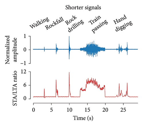
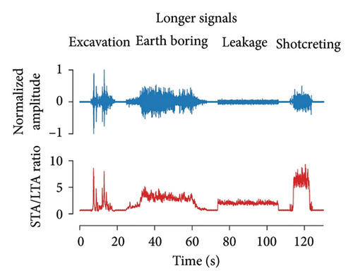
The dual thresholds of the STA/LTA ratio—which compares the average energy in an STA leading window to that in an LTA trailing window—are key to the robustness of the algorithm. To determine the base value for the upper threshold, we scrutinized the triggered STA/LTA ratio for all 1,494 samples of our dataset. The minimum ratio was set as the upper threshold, rounded down to 2.0. Based on the background noise level recorded by DAS in the Jing–Xiong intercity railway tunnel at 12:00 a.m. on July 28, 2020, UTC + 8 (details of the monitoring campaign are presented later), we chose 0.8 as the low threshold and a 5-second background noise as the standard noise. To extract the detected signals from the ambient vibration recordings while discarding unwanted data, we used the normalized cumulative energy curve, which allowed us to separate the signals of interest from the background noise in real time (Figure 4). Nine different types of tunnel disturbances captured by the anomaly detection pipeline are depicted in Figure 5, showing that even very low amplitude signals can be successfully detected.
4.2. Top Denoiser Evaluation
The side-to-side comparison of four denoisers (Figure 6) showed that CEEMD performed better overall in terms of SNR and RMSE, followed closely by VMD. For smoothness, EMD was superior to the other methods. VMD and WTD did not perform particularly well as expected. VMD, as the name implies, depends heavily on parameter tuning, especially the number of intrinsic mode functions, which varies with events. However, the mode number had to be fixed in the system (four, determined by a trial-and-error procedure), which caused under- or over-decomposition of certain types of signals, thus reducing the overall denoising performance. For WTD, the selection of wavelet function is an important factor affecting the algorithm performance. Here, we adopted a common parameter configuration of WTD: Daubechies extremal phase wavelets (db3), soft threshold, and four-level decomposition. Although a four-level wavelet decomposition can easily distinguish sharp signals from noise (e.g., rockfalls and walking), the small vanishing moment of db3 could make the signal unsmooth, leading to some loss of frequency-domain details, which explains WTD’s relatively poor smoothness metrics in some event categories.
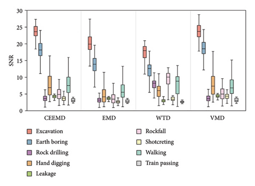
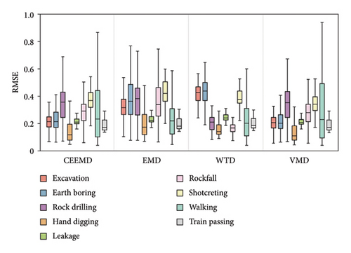
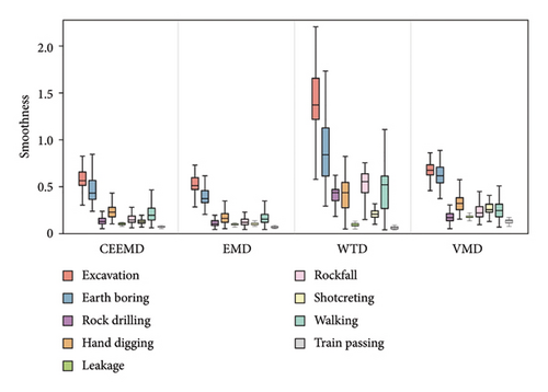
Based on the above performance evaluation, we excluded WTD because of its poor performance on all three metrics and EMD as it improves the smoothness by severely compromising SNR. Both CEEMD and VMD have excellent generalization capability, but the former can achieve relatively better denoising while requiring less computation time. Therefore, we finally chose CEEMD as the top denoising method for the nine tunnel anomalous signals. In addition, our results suggest that the number of tunable parameters plays a particularly important role when selecting a denoising method for multiclass vibration signals. Filters with fewer parameters usually have stronger transfer ability and therefore perform better overall on multiclass signals. In contrast, filters that rely extensively on parameter adjustment, such as VMD and WTD, are better suited for denoising specific vibration events.
4.3. Common Feature Set
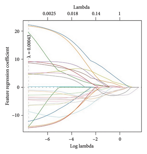
We first examined the relative importance of the 24 features for event recognition using elastic-net regression. To avert inflated performance evaluations due to overfitting, we split our dataset into a training set and a test set using a 7:3 ratio. Briefly, a threefold cross-validation procedure was used to determine the best values of two key elastic-net model parameters (alpha = 0.2, lambda = 0.00043) (Methods). Figure 7(a) shows how the regression coefficients calculated by elastic-net dynamically shrink with lambda; each line indicates the shrink trend of the coefficient of a specific feature. We graphed a feature importance chart according to the regression coefficients at the optimal lambda value 0.00043 (Figure 7(b)). We find that the total importance of the waveform and spectral features reached 75.29% (45.17% + 30.12%), indicating that the differences between the various types of tunnel vibration signals are mainly in their time- and frequency-domain features.
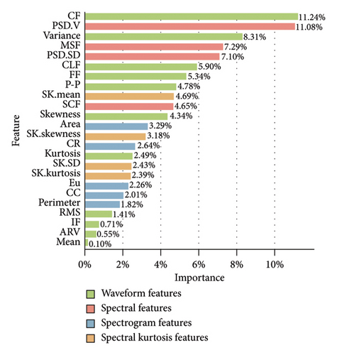
The most important feature for classification is crest factor (11.24%), a metric with high separation ability for impulsive signals (i.e., signals of large magnitude that occur over a short time interval). Interestingly, in the second and third places are both variance-related features: variance of normalized power spectral density (11.08%) and variance of wave amplitude (8.31%). Variance is a statistical measure of how discrete data points differ from the mean. The fact that two of the top three features are associated with variance indicates that our elastic-net model found signal variability to be the most useful in differentiating between different events. The importance of spectrogram and spectral kurtosis features is relatively low, accounting for 12.02% and 12.69%, respectively. They were included in the feature vector to enrich the variety of feature categories and improve the predictive power.
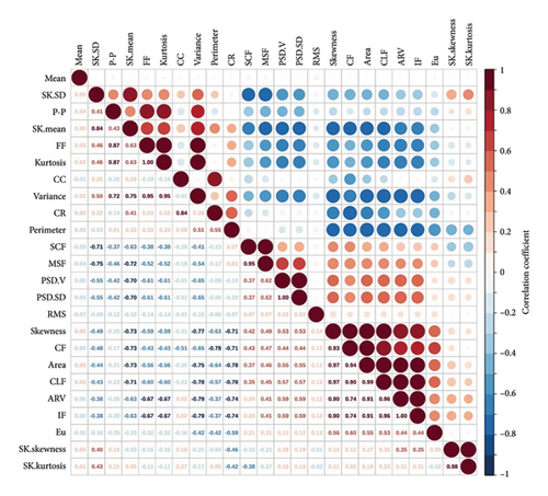
Multicollinearity among independent variables can lead to unreliable predictions [41]. To avoid collinearity and reduce the dimensionality of our feature space, we combined heatmap correlation analysis with the feature importance to filter out features that are statistically highly intercorrelated and of relatively low importance for recognition. According to the feature-correlation heatmap (Figure 7(c)), skewness was excluded because it is highly correlated with area (r = 0.97), clearance factor (r = 0.97), and crest factor (r = 0.93). Clearance factor has a high correlation of r > 0.9 with crest factor or impulse factor, and all three features are sensitive to impulsive signals, so we removed clearance factor to reduce multicollinearity. The average rectified value is linearly correlated with impulse factor (r = 1); we retained the latter for its slightly higher importance score. Variance, form factor, and kurtosis are three highly intercorrelated features; we kept only variance to optimize the feature space. Because mean had little importance for classification (0.1%), it was removed to reduce computational efforts. In total, we selected five waveform features. Likewise, multicollinearity correction and dimensionality reduction were performed for the other three feature categories considering both feature correlation and feature importance. Combining heatmap correlation analysis and elastic-net regression, we removed nine features with statistically high intercorrelation or of relatively low importance, leaving 15 predictive features (features 2, 4, 7, 9, 10, 12, 14, 16–20, and 21–23 in Table 2) for downstream machine learning and pattern recognition. For each detected signal, our feature extraction module generates a vector containing 15 feature values for downstream pattern recognition.
To illustrate how dimensionality reduction quantitatively improves the recognition ability of our final stack model, we used the dataset of 24 and 15 features, respectively, to train the model using a threefold cross-validation, optimized with PSO. The results show that feature selection improves the accuracy, precision, recall, and F1-score by 1.34%, 1.70%, 0.71%, and 1.21%, respectively (Figure 8).

4.4. Multiclass Classification Results
4.4.1. Base Classifier Selection
We compared 10 classification algorithms that cover a variety of popular methods for machine learning. According to the algorithm principle, LSTM is a deep learning method with some memory effect and is suitable for processing time-series data with massive variables. We excluded LSTM because it is poorly interpretable with many tunable parameters, which was considered unsuitable for the current supervised multiclassification task. We removed the PNN and BP algorithms because they have been incorporated into other algorithms as basic methods. For example, the gradient transfer method in the MLP algorithm is based on the idea of BP.
We evaluated the remaining seven classifiers on a performance basis. A threefold cross-validation framework was implemented, and PSO was used for optimization (Table 6). According to a side-to-side performance comparison as well as considering their algorithmic characteristics (Table 7), we selected five well-performing models as our base classifiers: SVM, XGBoost, RF, LR, and KNN. We chose LR as our meta classifier to combine the predictions from the base classifiers.
| Base classifier | Hyperparameter | Explanation |
|---|---|---|
| SVM | C = 22.4690 | Coefficients of the L2-norm |
| Gramma = 5.9034 | Kernel coefficient | |
| LR | C = 50 | Reciprocal of the coefficients of L2-norm |
| KNN | n_neighbors = 3 | Number of neighbors (K value in KNN) |
| MLP | hidden_layer_sizes = 50 | Number of neurons in the hidden layer |
| Alpha = 0.1 | Coefficients of the L2-norm | |
| NB | var_smoothing = 1.00E − 06 | Portion of the largest variance of all features |
| RF | n_estimators = 70 | Number of decision trees |
| max_depth = 10 | Maximum depth of decision tree | |
| XGBoost | n_estimators = 100 | Number of decision trees |
| max_depth = 3 | Maximum depth of decision tree | |
- Abbreviations: KNN, k-nearest neighbor; LR, logistic regression; MLP, multilayer perceptron; NB, Naive Bayes; RF, random forest; SVM, support vector machine; XGBoost, eXtreme gradient boosting.
| Model | Accuracy (%) | Precision (%) | Recall (%) | F1-score (%) |
|---|---|---|---|---|
| SVM | 96.44 | 96.70 | 95.68 | 96.15 |
| LR | 94.43 | 93.18 | 94.64 | 93.74 |
| KNN | 94.21 | 95.04 | 93.34 | 93.99 |
| MLP | 89.98 | 86.80 | 88.62 | 87.38 |
| NB | 87.31 | 85.57 | 88.49 | 85.56 |
| RF | 93.76 | 94.08 | 93.48 | 93.70 |
| XGBoost | 95.99 | 96.21 | 95.04 | 95.56 |
- Abbreviations: KNN, k-nearest neighbor; LR, logistic regression; MLP, multilayer perceptron; NB, Naive Bayes; RF, random forest; SVM, support vector machine; XGBoost, eXtreme gradient boosting.
4.4.2. Stacking Model Performance Evaluation
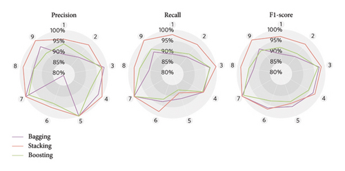
To examine whether stacking improved the classification ability of the machine learning model, we benchmarked the performance of our model against two other ensemble strategies: boosting and bagging. We built three stacking models: stacking_E1 is our final model with SVM, XGBoost, RF, LR, and KNN as the base classifiers; stacking_E2 is essentially stacking_E1 plus MLP and NB; and stacking_E3 removes XGBoost and RF from stacking_E2. LR is the meta classifier for all three stacking models. Again, we implemented a threefold cross-validation framework with hyperparameter tuning using PSO. We graphed the evaluation results by algorithm type (Figure 9(a)) and event category (Figure 9(b)). For simplicity, we used Categories 1–9 to represent, in order, excavation, earth boring, rock drilling, hand digging, water leakage, rockfall, shotcreting, walking, and train passing.
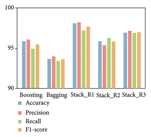
The comparison with the test set demonstrated that our stacking model (stacking_E1) had better overall (macro) performance than boosting, bagging, and the other two stacking models in classifying various tunnel disturbances (Figure 9(a)). For example, our stacking model had a macro-accuracy of 98.22%, which was 2.23% higher than boosting and 4.46% higher than bagging. With five good classifiers in the ensemble, stacking_E1 achieved a 1.12% higher accuracy than stacking_E3. In addition, increasing the number of base classifiers does not necessarily improve the model’s recognition ability. For example, stacking_E1 with only five classifiers outperformed stacking_E2 with seven classifiers due to the poor performance of the added MLP and NB. This emphasizes the importance of base-classifier selection for ensemble learning models.
This evaluation also showed that stacking_E1 scored higher on almost all individual event categories than other models (Figure 9(b)). Our trained model was the most precise in recognizing eight event categories except for rock drilling (Category 3), on which it scored 97.59%, only 0.96% less precise than bagging. In terms of recall and F1-score, our model scored lower than bagging only in water leakage (Category 5), with a difference of 2.78% (recall) and 1.53% (f1-score), respectively.
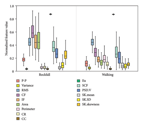
Of the eight event categories, rockfall (Category 6) is not only among the most crucial monitoring target from a geotechnical perspective but also the least reliably identified. Our model recognized rockfall with an F1-score of 96.91% (the second lowest F1-score), compared to 100% for shotcreting (Category 7) and train passing (Category 9). This low F1-score is mainly due to the high overlap of the spectral kurtosis feature SK.SD (sensitive to impulsive signals) between rockfall and walking (Category 8) (Figure 10(a)), both characterized by short-duration impulsive attributes. Another observation is that excavation was identified with an equally low F1-score (96.91%). This is because the excavation signal closely resembles the earth boring signal (Category 2) in the time–frequency domain binary image, leading to an overlap of the features Eu and CR describing the outline of the binary image (Figure 10(b)), which is likely to cause misclassifications.

In summary, this side-to-side comparison proves the ability of the trained stacking ensemble learning model to correctly recognize multiple tunnel disturbances and also supports that stacking can harness the capabilities of sub-models on classification tasks.
5. Real-World Application
In order to verify the efficacy and transferability of our tunnel threat monitoring system, we carried out a 1-month DAS monitoring experiment at the Jing–Xiong intercity railway tunnel (Gu’an County, Hebei Province, China) (Figure 11). The test tunnel is a single-hole, double-line tunnel with a full length of 7208 m, a width of 15 m, a shallow depth of 8 m, and a maximum depth of 22 m (Figure 12). We deployed a 2-mm diameter single-mode fiber-optic cable (tight-buffered, thermoplastic polyurethane-jacketed) with a total length of 8000 m in this tunnel, which can be roughly divided into two sections. The first 4530 m of the cable was laid near the central water ditch at the bottom of the tunnel to monitor events such as rockfalls, machinery operations, and train passing. The rest of the cable were laid on top of the tunnel for intrusion and water leakage detection. The coupling between the fiber and the surrounding medium is a key factor for the successful fiber-optic monitoring [45, 46]. To ensure optimal tunnel-to-fiber coupling, we directly embedded the pretensioned cable into the groove on the sidewall of the ditch and then fixed it with epoxy resin adhesive every 1 m (Figure 12(b)). For the tunnel roof section, the surface-bonding method was used to fasten the cable to the tunnel segments (Figure 12(c)). Finally, the roof cable section and the ground cable section were fused at one end of the cable, while the other end was connected to a DAS integration unit (IU). Continuous vibration measurements were made by the DAS IU at a 2000-Hz sample rate with a 10-m channel spacing from August 1, 2020, to August 31, 2020, UTC + 8.
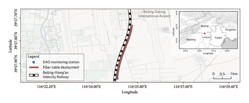
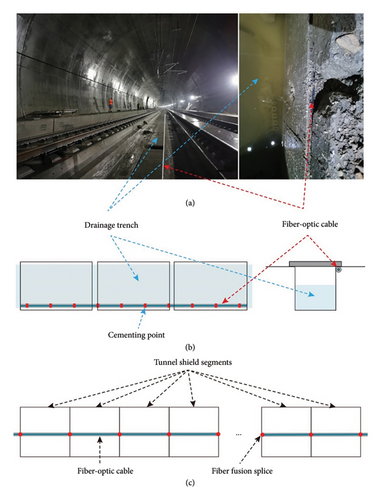
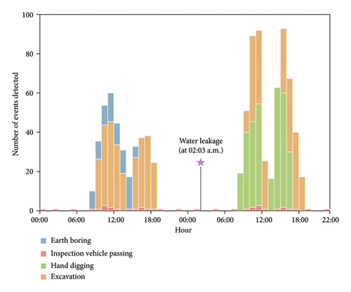
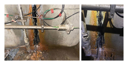
Figure 13 shows the disturbance events detected by DAS on August 29 and 30. During the 2-day monitoring period, our intelligent DAS system identified a range of tunnel disturbances, including excavation, earth boring, and inspection vehicle passing. Furthermore, the number of events recognized was highly consistent with the manual inspection record on site. In addition, our monitoring system successfully captured a small-scale water leakage event in the early morning (2:03 a.m.) of August 29. Manual inspection confirmed that it was caused by cracking of the concrete tunnel lining (Figure 14), which, if not detected in time, might develop into a larger-scale water inflow.
6. Discussion and Conclusions
We have shown how machine learning methods can be paired with the emerging DAS technology to automatically identify a variety of anomalous vibration events that threaten underground tunnels. Through a real-world application in the Jing–Xiong railway tunnel, we demonstrate how such automated monitoring enables the timely detection of weak-energy but highly dangerous events, such as water leaks. In contrast to traditional node-based microseismic monitoring methods that typically deal with specific tunnel hazards (e.g., rock bursts [47]), our intelligent surveillance system leverages the long-range sensing capability, dense spatial sampling strength, and broadband nature of DAS, thus being able to extend over tens of kilometers and detect a wide range of tunnel threats. Our stacking ensemble model integrates multiple classifiers for automatic feature learning, improving adaptability, robustness, and detection accuracy in diverse tunnel disturbance events. Furthermore, the sensing fibers—slender yet robust—can be easily deployed in confined spaces and are highly durable in subsurface environments, allowing for long-term tunnel safety monitoring. Additionally, passing trains are potential sources of vibration. With ambient noise tomography techniques [48], the passively recorded multichannel background noise can be exploited to image high-resolution stratigraphic structures around tunnels. Together, these could open up new possibilities for tunnel and underground space research.
Our work also represents an important step forward in the development of a general framework for processing and efficiently exploring sizable volumes of engineering DAS data. Several artificial intelligence–based approaches [25–29] using site-specific DAS datasets have been proved to achieve high local accuracy, but they lack transferability between sites. By contrast, the current machine learning model is highly transferable thanks to the good generalization ability of stacking ensemble learning, and most importantly, it has been trained with high-quality vibroacoustic data collected in real tunnel environments that span tunnel types, soil conditions, and geographical conditions. Moreover, selected from 24 typical signal features, our 15-dimensional feature set is exceptionally descriptive across diverse tunnel disturbances—from geologic hazards such as rockfalls and groundwater inflows to machinery operations and regular train passing. In addition, the remarkable efficacy of the automatic anomaly detection pipeline provides a universal solution for picking, separating, and denoising anomalous signals. Hence, our machine learning–based autonomous DAS monitoring approach is highly generalizable and can be well transferred to new and vastly differing tunnel environments. However, we recognize that the performance of our model could be limited by the diversity of event types in the training data. When event types not included in the training set occur, the detection accuracy may decrease significantly due to the model’s difficulty in interpreting unfamiliar patterns. Therefore, our next work is to improve the model’s adaptability to unknown events by employing advanced open-set algorithms and increasing the volume of training data. As more datasets become available, we anticipate that the intelligent DAS monitoring system will be able to be refined and deployed in a wide variety of underground spaces.
Conflicts of Interest
The authors declare no conflicts of interest.
Funding
This work was supported by the National Natural Science Foundation of China grants (grant numbers 42030701 and 42107153), the Natural Science Foundation of Jiangsu Province grant (grant number BK20200217), and the Yuxiu Young Scholars Program of Nanjing University (grant number 2010619).
Acknowledgments
We are grateful to Jun Yin, Zheng Wang, Jun-Peng Li, and NanZee staff for contribution to the development of the dataset and for assistance in the field monitoring campaign. We thank Dechuan Zhan and Su Lu for advice on building the machine learning model and Zheng Wang for assistance in drawing Figure 11.
Open Research
Data Availability Statement
The data that support the findings of this study are available from the corresponding author upon reasonable request.


