Seepage is one of the main causes of dam accidents, characterized by long latency periods and spatiotemporal randomness. In this study, an innovative combined algorithm model (AT-LSTM-CUSUM) is proposed to predict such leakage hazards. First, a long short-term memory (LSTM) network model based on an attention mechanism is established to focus on key influencing factors in predicting the time series data. Following the time series prediction, an improved Cumulative Sum (CUSUM) change-point monitoring algorithm is introduced. Within a sliding window period, a control function collects cumulative residuals, and a threshold test is performed to determine whether a potential hazard trend exists. Using monitoring data from a pressure measuring pipe in a concrete dam as the experimental subject, five related influencing factors were collected (upstream and downstream water levels, temperature, precipitation, and structural aging). These data were fed into the AT-LSTM model for iterative parameter tuning, yielding optimal prediction results. These results were compared with those of the LSTM, GRU, ARIMA, and Prophet models, validating the superior performance of the AT-LSTM model. In addition, by simulating the seepage hazard occurrence process, the change-point monitoring effectiveness of the improved CUSUM algorithm was tested. A parameter sensitivity analysis of the window period and threshold values revealed that the algorithm performed effectively in detecting seepage hazards. The innovative algorithm proposed in this paper exhibits strong early warning capabilities and holds significant value for dam safety monitoring and maintenance.

1. Introduction

Seepage is one of the main causes of dam accidents [1]. In recent years, dam accidents caused by seepage have become frequent, accounting for about 29.1% of dam failures, with 2344 at-risk reservoirs experiencing leakage issues [2]. For example, in July 2024, a severe seepage hazard occurred at the Jiufeng Reservoir dam in Hunan Province, China. Water seeped from a conduit at an elevation of 98 m (with the reservoir water level at 125.30 m). The seepage was detected by inspection personnel when significant water leakage was observed at the dam’s drainage prism toe, and timely emergency measures successfully controlled the hazard.

For such concealed seepage hazards, relying solely on manual inspections or sampling methods poses significant risks. In addition, current sampling detection methods typically rely on traditional laboratory or on-site experiments, which are costly, invasive, and time-consuming. With the growing application of intelligent technologies in dam monitoring [3], many researchers have combined these technologies with mathematical prediction models to forecast changes in dam seepage data. These methods include ARIMA time series, Prophet, support vector machine (SVM), BP neural networks, and extreme learning machines [4–14]. While these algorithms perform well in predicting dam seepage data under normal conditions, there is still a lack of research on predicting and providing timely warnings for concealed seepage hazards caused by sudden events (such as floods or earthquakes) or internal structural erosion and damage.

To address these concealed seepage hazards with spatiotemporal randomness, this paper proposes a solution that involves deploying sensors in weak areas of the dam to collect seepage data in real time. The improved combined algorithm AT-LSTM-CUSUM is then used to predict seepage data, addressing both normal seepage predictions and potential leakage accident warnings, thereby achieving real-time monitoring of dam seepage safety.

2. The Principles of the AT-LSTM-CUSUM Seepage Prediction Model

2.1. Principles of the AT-LSTM Model

2.1.1. Principles of Long Short-Term Memory (LSTM)

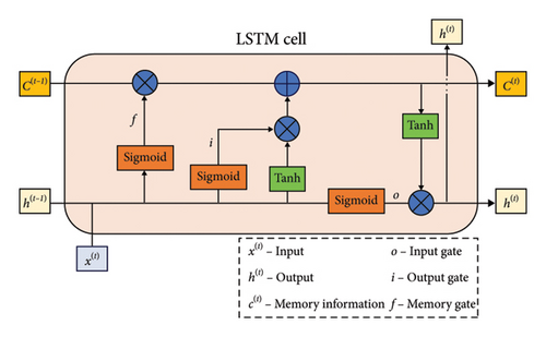
LSTM networks, compared with traditional neural networks, can effectively solve the forgetting problem and extend the time unit of the processed time series data. The core idea is to construct cell units that selectively remember important information based on the internal dependencies of time series, filtering out noise and reducing memory burden. The structure of LSTM includes three types of gating mechanisms: the input gate, output gate, and forget gate. The output vector of the model is divided into the current state vector and the output vector. The inputs consist of the state vector of the previous time step, the output vector of the previous time step, and the input vector of the current time step [15].

The calculation formulas for each cell unit are as follows:

(1)

where W represents the weight matrix and b is the bias vector. The σ(sigmoid) function outputs values between 0 and 1, allowing for the elimination of zero elements during matrix multiplication, effectively functioning as a forget gate that selectively forgets certain memories. The tanh function, which ranges from −1 to 1, is used to condense and organize information.

The schematic diagram of the LSTM cell structure is shown in Figure 1:

Details are in the caption following the image — **Figure 1**
Open in figure viewer PowerPoint

Schematic diagram of the LSTM cell structure.

2.1.2. Attention Mechanism

LSTM is proficient at handling time series data and capturing dependencies within sequences, selectively remembering important internal information. However, it gives equal attention to all external input features, which affects prediction accuracy. Therefore, the attention mechanism is introduced, much like installing a focusing device in data processing. It allocates different weights to factors based on their importance to leakage, thereby highlighting the key influencing factors [16].

The attention mechanism involves three input vectors.

The Q(Querry), used to retrieve correlations with other variables, the K(Key), reflecting the degree of association between the corresponding input elements and the query vector, and the V(Value), which contains the actual data information [17].

The operational steps are as follows:

1.
Data encoding: transform the input data into corresponding 〈K, V〉 pairs using appropriate encoding.
2.
Calculating relevance: determine the correlation between the query vector and each key vector. After normalization, obtain the attention weights corresponding to each input element.
3.
Weighted information aggregation: perform a weighted summation of each value vector based on the weight coefficients.

Attention weight coefficient W:

(2)

Output after processing by the attention mechanism:

(3)

2.1.3. LSTM Network Based on the Attention Mechanism

The model framework is illustrated in Figure 2, comprising the input layer, hidden layer, attention layer, fully connected layer, and output layer.

Input layer: accepts multidimensional time series data and transforms its format.
Hidden layer: consists of multiple LSTM cell units that process the time series data.
Attention layer: computes the attention distribution at different time points.
Fully connected layer: transforms the data and performs local integration.
Output layer: delivers the prediction results.

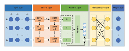
By introducing the attention mechanism, the model dynamically focuses on the importance of various factors at different time points, disregards irrelevant information, and emphasizes key data. This integration into the memory network can enhance the model’s predictive performance [18].

2.2. Improved Cumulative Sum (CUSUM) Algorithm

Dam leakage issues typically have a long latency period, and the changes in leakage behavior are often slow and covert [19]. Traditional anomaly detection methods struggle to effectively identify potential risks in the early stages. For example, factors such as water level fluctuations caused by precipitation, temperature changes, or gradual structural erosion can lead to small and slow changes in seepage flow, which often accumulate gradually without noticeable abrupt shifts. To address this challenge, an anomaly detection method capable of efficiently and sensitively capturing these progressive changes is needed. General time series anomaly detection can be based on predictive data [20]. In this paper, an innovative approach is taken by using the residuals between reasonable predicted values and actual values to assess anomalies in advance, based on a deep integration with the research problem background [21]. The residuals obtained by subtracting the actual seepage pressure values from the reasonable values predicted by the AT-LSTM model are introduced into the improved CUSUM algorithm for change point detection.

2.2.1. Algorithm Principle and Improvement Plan

The CUSUM algorithm [22] is a statistical control method used to detect changes in the mean of a process, and it has been widely used in engineering monitoring fields [23]. The principle is to continuously calculate the cumulative sum of the deviation between the observed values and the target or reference values. When the cumulative sum exceeds the preset control limit, it indicates a significant change in the process mean, suggesting the potential presence of an anomaly. Its advantage lies in its sensitivity to small potential changes, allowing it to detect such changes relatively quickly [24]. It is effective for detecting gradual changes and change points in time series and can respond to potential data changes, providing early warnings. However, the traditional CUSUM algorithm is mainly suitable for detecting abrupt changes in data and is not effective for the slow changes or progressive anomalies commonly found in dam seepage monitoring. Dam seepage changes are usually subtle and slow, influenced by factors such as water level, precipitation, and temperature. The traditional CUSUM algorithm is ineffective at capturing these small, gradual changes. Therefore, this paper proposes an improved CUSUM algorithm. The improvement plan is mainly optimized in the following three aspects:

Residual calculation: replace the mean change in the original CUSUM algorithm with the residuals between predicted and actual values. In this way, the algorithm can focus on capturing the deviation between seepage flow and reasonable predicted values, thereby mitigating the influence of external factors (such as climate or precipitation) that cause periodic fluctuations. This makes the residuals better reflect anomalies caused by structural issues or potential leakage.
Sliding window: we innovatively introduce a sliding window mechanism, ensuring that each monitoring node triggers a monitoring cycle, taking into account the dam’s historical data rather than relying solely on anomaly points for triggering, thus achieving real-time monitoring of leakage safety.
Control function: the established control function effectively manages the acceptance level of seepage data, enhancing the system’s noise resistance and change-point sensitivity. For continuously fluctuating positive residuals, the system gradually increases the acceptance level; for occasional discontinuous errors, it filters and selects based on the fluctuation amplitude, ensuring more accurate and reliable detection results.

2.2.2. Implementation Process of the Improved CUSUM Algorithm

The detailed algorithm visualization is shown in Figure 3, and the following text describes the specific algorithm process.

1.
Use the AT-LSTM model to predict the seepage data for the next period in real-time, followed by actual measurements of the seepage data during that period.
(4)
where i represent the monitoring time units starting from the initial monitoring point, measured in days.
2.
Starting from the initial monitoring point, calculate the difference between the reasonable predicted data y_gt(i) and the actual measured data y_pv(i) at each time point from (1). The residual value is denoted as Δy_(i).
(5)
3.
Each time a new measurement time point is reached, initiate a new monitoring window cycle T_new from that time point Δy_new.
(6)

If, within the specified period following that time point, the cumulative value of positive residuals

does not reach the warning threshold S_upper, the cumulative value is reset to zero, and that window exits.

(7)

If the cumulative residual value reaches the warning threshold, a warning report is triggered, indicating the potential development of a risk situation.

(8)

where T be the sliding monitoring window period. Considering the concealed nature and long incubation period of seepage risks, the initial monitoring cycle is set to 100 days, although this specific value needs to be adjusted based on the dam and local hydrological conditions, where S_upper be the cumulative residual threshold. Following the classical principle 3σ in statistics, the threshold can initially be set as a multiple of three standard deviations; again, the optimal value should be adjusted according to actual conditions.

represents the positive residual, which refers to the collected measured values that exceed the predicted values, focusing solely on anomalies related to excessive seepage.

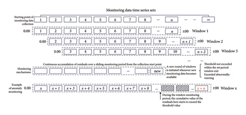
Let A(t) denote the acceptance function, which dynamically adjusts the acceptance levels to enhance noise resistance and sensitivity to change points. Continuous fluctuations in positive residuals receive sufficient attention, with increasing sensitivity and progressively higher acceptance levels. In contrast, a filtering function is applied to sporadic residuals, where the acceptance level is related to the size of the residual. Small fluctuations in sporadic residuals are accepted, while larger fluctuations result in progressively lower acceptance.

The constructed acceptance function and illustrations are presented in equation (9) and Figure 4.

(9)

where A(t) is the acceptance level of the residual at time point, R(t) is the residual at time point, R(t) = Δy_(i) is the increment in acceptance level for continuous positive residuals, and e^−R(t) is the control function for sporadic discontinuous residuals.

3. Engineering Case Study

3.1. Data Collection and Processing

The case study is the Ertan Hydroelectric Station in Panzhihua City, Sichuan Province, China, where the hydraulic hub is a concrete double-curvature arch dam [7]. The research data consist of the piezometric levels measured by the piezometer in the dam’s impermeable curtain from 2011 to 2019. We selected measurement point A as the primary point for pressure prediction research and introduced data from two other points, B and C, for model validation, which are shown in Figures 5 and 6.

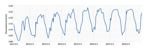
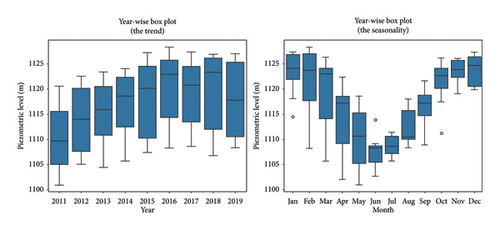
From Figure 7, it can be observed that the seepage pressure data exhibits annual periodicity, with values ranging from (1100.893 to 1128.329) m. It can be indirectly inferred that the seepage amount shows a slight year-on-year increase but remains generally stable. The data distribution is skewed, with a significant degree of dispersion, and the peak seepage primarily occurs from May to October each year.

The following are the relevant independent variables selected based on the research analysis [7, 25]:

(10)

3.1.1. Data Preprocessing

In this study, outliers are handled using the box plot method, missing data are filled using linear interpolation, and all data are normalized to the range of 0-1 using the following equation.

(11)

1.
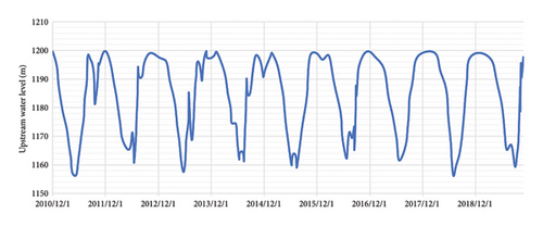
Upstream water volume (X_upstream): the higher the upstream water level, the greater the seepage pressure on the dam structure, which leads to more water leaking through the dam. Figure 8 shows the upstream water level variation data of the dam over the past 9 years.
2.
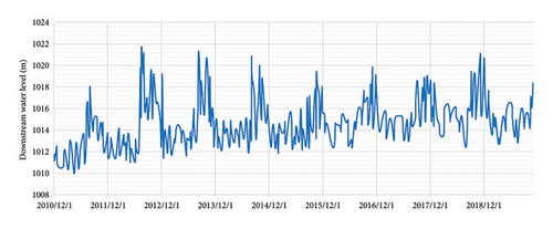
Downstream water volume (X_downstream): the lower the downstream water level, the greater the seepage pressure differential, which may increase leakage. Figure 9 shows the 9 years of downstream water level variation data for the dam.
3.
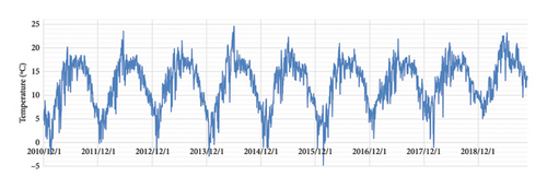
Temperature (X_temperature): fluctuations in temperature cause thermal expansion and contraction in concrete dams, which can lead to cracks that provide pathways for seepage. In addition, low temperatures can cause pore water within the dam to freeze and expand, further damaging the structure and increasing the likelihood of seepage. Figure 10 shows the daily average temperature variation data at ground level.
4.
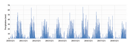
Precipitation (X_{precipitation}): precipitation increases the water content around the dam, leading to higher mountain runoff, which raises the upstream water level and increases the risk of seepage. Intense precipitation can rapidly alter the hydrological conditions around the dam, potentially causing peak seepage events over a short period. Moreover, precipitation infiltrating the dam may alter the infiltration line (i.e., the depth at which water enters the dam body), which not only increases the likelihood of seepage but may also destabilize certain sections of the dam, further exacerbating leakage. Figure 11 shows the daily rainfall variation data for the region.
Furthermore, considering the lag effect of precipitation, a delagging time series is introduced to minimize this impact [26]. The specific operations are as follows:
(12)
where ρ_XY(k) is the cross-correlation coefficient between precipitation X_t and seepage Y_t at lag k; Cov(X_t, Y_t+k) is the covariance between precipitation and seepage at lag are the mean values of precipitation and seepage, respectively; and σ_X and σ_Y are the standard deviations of precipitation and seepage, respectively.
- a.
  Identify the lag with maximum correlation: determine the time lag that corresponds to the highest cross-correlation between precipitation and seepage.
  (13)
- b.
  Delagging process: shift the precipitation sequence X_t forward by k^∗ time units to generate the delagged precipitation sequence , aligning it with the seepage data Y_t.
Section 3.4 will explore the impact of rainfall lag treatment on dam prediction results.
5.
Aging of structural facilities (X_aging):
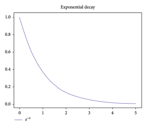
As time progresses, the aging of dam structures becomes apparent, manifested by the growth and extension of cracks and the failure of water-stopping facilities, all of which contribute to increased seepage. The initial aging of the dam occurs relatively rapidly, primarily due to material degradation and the formation of microcracks. However, the aging rate slows down over time. To more accurately describe this process, a logarithmic decay model is often used. This model indicates that crack extension and the degradation of water-stopping facilities follow a logarithmic decay, with rapid aging in the early stages and a gradual stabilization over time.
(14)
where t is the number of days since the dam started operation, C(t) is the dam’s operational capacity at time t (ranging from 0 to 1), C₀ is the dam’s initial operational capacity (set to 1), and α is the aging rate coefficient, which controls the rate of aging (considering that the monitoring data was collected from a dam that has been in operation for 20–30 years and is now in the aging phase, the value of α is set to 0.2).

3.2. Seepage Pressure Prediction Results

A multivariate time series prediction model is established, with the five types of influencing factor datasets from the previous section imported. The seepage pressure data are divided into a training set and a test set (with the last 10% used as the test set). After cross-validation and continuous iterative adjustment using the Adam algorithm for optimization, the optimal training results are shown in Figure 12 and Table 1.

(15)

Table 1. Evaluation of AT-LSTM model predicted seepage pressure data for three measurement points.

Measurement point	Evaluation metrics	Train	Test
Point A	Root mean square error (RMSE) (m)	0.2659	0.3725
	Mean absolute error (MAE) (m)	0.1568	0.4511
	Coefficient of determination (R²)	0.9913	0.9766

Point B	Root mean square error (RMSE) (m)	0.3026	0.5075
	Mean absolute error (MAE) (m)	0.2254	0.5578
	Coefficient of determination (R²)	0.9856	0.9733

Point C	Root mean square error (RMSE) (m)	0.2018	0.2241
	Mean absolute error (MAE) (m)	0.1346	0.4059
	Coefficient of determination (R²)	0.9945	0.9856

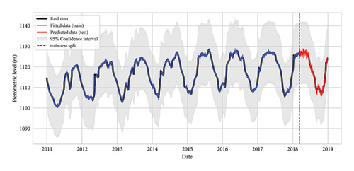
Based on the evaluation metrics and graphical visualization, it is clear that the AT-LSTM model demonstrates excellent predictive performance for the variations in seepage pressure data, effectively forecasting changes in dam seepage pressure.

3.3. Comparison With Prediction Results From Four Other Models

A comparative evaluation was conducted between the improved model and LSTM, Random Forest, and two univariate prediction models (ARIMA and Prophet). As shown in Table 2, on the test set, the AT-LSTM model improved the R² by 4.7%, 3.5%, 14.7%, and 14.3% compared with the LSTM, GRU, ARIMA, and Prophet models, respectively, verifying the accuracy of AT-LSTM.

Table 2. Comparison of evaluation metrics for different models.

Measurement point	Model	Training set			Validation set
Measurement point	Model	RMSE	MAE	R²	RMSE	MAE	R²
Point A	AT-LSTM	0.266	0.157	0.991	0.373	0.451	0.978
	LSTM	2.055	1.854	0.902	1.052	0.931	0.934
	GRU	3.579	3.112	0.918	2.036	1.878	0.945
	Prophet	10.524	6.539	0.913	4.255	2.987	0.853
	ARIMA	23.891	13.524	0.875	15.297	9.032	0.856

Point B	AT-LSTM	0.303	0.225	0.986	0.508	0.558	0.973

Point C	AT-LSTM	0.202	0.135	0.995	0.224	0.406	0.986

3.4. The Impact of Rainfall Lag Treatment on Dam Prediction

By solving the lagged time series, we obtain the maximum correlation lag periods k^∗ for three measurement points (A, B, and C), which are 6.3 days, 5.5 days, and 7.0 days, respectively. We compare the results before and after applying lag treatment in the model to explore the impact of lag handling on the prediction model. The specific details are shown in Table 3.

Table 3. Evaluation of the impact of lag on model prediction performance.

Measurement point	Lag period (days)	R² of the prediction after lag treatment	R² of the prediction without lag treatment
Point A	6.3	0.978	0.968
Point B	5.5	0.973	0.970
Point C	7.0	0.986	0.971

As shown in Table 3, lag treatment has improved prediction accuracy to some extent, with this effect being more evident at measurement point C. Although the overall impact is not very high (likely because the weight of rainfall in the prediction model is relatively low), it reflects the existence of the lag effect of rainfall on dam seepage.

3.5. Analysis of Attention Weights for Each Factor

In fact, the impact of various external factors on dam seepage differs across periods, but the weights recognized by general prediction algorithms are mostly fixed. The AT-LSTM model addresses this issue effectively. With the intervention of the attention mechanism, it can dynamically adjust the weights of each influencing factor at different time steps, thereby improving the model’s prediction accuracy. Given the long time span of the overall data, for clearer presentation, this paper uses measurement point A as an example and selects data from 2016 to 2017 to demonstrate the dynamic changes in attention weights by month, which is shown in Figure 13.

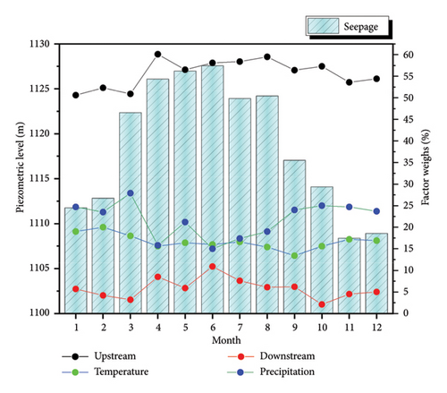
The figure compares the changes in weights for four influencing factors and seepage (the aging factor is not discussed here due to its low contribution to the model). It can be seen that the attention weights of these four influencing factors change dynamically over time. The upstream water level consistently holds a significant weight on seepage, fluctuating between 50% and 70%, while the downstream water level has a much smaller impact, with its weight remaining below 10%. Meanwhile, the weight of rainfall is slightly higher than that of temperature, and the weight variations for the four factors remain generally stable. Interestingly, during the local flood season (May–August), which coincides with the peak of dam seepage, the impact weights of upstream and downstream water levels increase, reflecting that water level may be a more direct factor influencing dam leakage.

3.6. Testing the Early Warning Effectiveness of the Simulated Risk

3.6.1. Determination of Parameters for the Improved CUSUM Algorithm

1.
Historical normal data are collected to analyze the distribution characteristics of the residuals, and it is found that the residuals approximately follow a normal distribution x ~ N(μ, σ²). Calculations show that the mean of the 100-day residual sample data is close to 0, with a standard deviation of approximately 0.068, which is shown in Figure 14.
2.
Considering that the residuals at each time point follow a normal distribution N(μ, σ²), when these residuals are accumulated, the cumulative residual S_n is composed of multiple independent normally distributed random variables as follows:
(16)

According to the central limit theorem, the cumulative residual S_n will also tend toward a normal distribution , with a mean μs = 0, and a standard deviation . Based on 3σ principle, there is a 99.73% probability that the cumulative residual threshold will fall within three standard deviations. We set the residual threshold to 3σ_s = 2.04, and this setting performs well in later tests.

3.6.2. Testing the Model’s Early Warning Effectiveness

By simulating a seepage risk scenario based on historical accident data, this study examines the effectiveness of the LSTM-CUSUM model for early warning, which are shown in Figure 15.

The results show that the algorithm, combined with LSTM predictions, can effectively identify gradual changes and provide early warnings for sudden risk trends. In the simulation, hidden seepage began around day 60, and the CUSUM model detected a significant trend change around day 72 through accumulated residuals. This provided a warning about 8 days earlier than traditional anomaly detection methods.

3.6.3. Comparison of Model Performance and Exploration of Reasons

The improved CUSUM model and other algorithms are compared and analyzed through multiple model experiments to evaluate their performance, and the results are shown in Table 4.

Table 4. Comparison of model effects.

Evaluation metrics	Improved CUSUM	Traditional CUSUM	DBSCAN	Isolation forest
Average warning time	12 days	11 days	20 days	16 days
Noise tolerance	High	Low	Moderate	Moderate
False alarm rate	< 10%	< 25%	< 10%	< 5%

The improved CUSUM and traditional CUSUM (with identical parameters but without control functions) are analyzed using the residual sequence, while other algorithms are analyzed using normally collected monitoring data. As shown in Table 4, the improved CUSUM algorithm effectively overcomes the shortcomings of the traditional CUSUM algorithm and outperforms other traditional anomaly detection models.

Reason analysis: in terms of early warning time, the improved CUSUM algorithm, by continuously accumulating prediction residuals, can promptly capture subtle changes in seepage, thus providing quicker anomaly alerts. Although traditional CUSUM can detect mean changes, it is less resistant to noise. DBSCAN and Isolation Forest, when dealing with gradually changing seepage data, often experience delayed warnings due to their high data distribution requirements. Moreover, in terms of robustness, the improved CUSUM can effectively filter out occasional noise and periodic influences (such as water level fluctuations and precipitation), focusing on anomalies caused by changes in the dam structure. This results in stronger stability in complex environments. In contrast, DBSCAN and Isolation Forest are more susceptible to noise interference, leading to false alarms.

3.7. Sensitivity Analysis of Improved CUSUM Parameters

Sliding window period: the window period in the CUSUM algorithm defines how many observations are used to accumulate the residuals. A smaller window period can respond more quickly to changes but may be affected by noise, leading to false alarms. A larger window period responds more smoothly to changes, reducing false alarms, but may delay the detection of anomalies.
Cumulative residual threshold: the choice of control limits (thresholds) determines the sensitivity of the algorithm. A smaller threshold can detect even small changes in the mean more sensitively, but it may increase the risk of false alarms. A larger threshold may miss smaller changes but reduce false alarms.

In the following, based on the reasonable parameters successfully validated earlier, we adjust these two parameters and observe the model’s response under different combinations : [T, S_upper], and the results are shown in Figure 16.

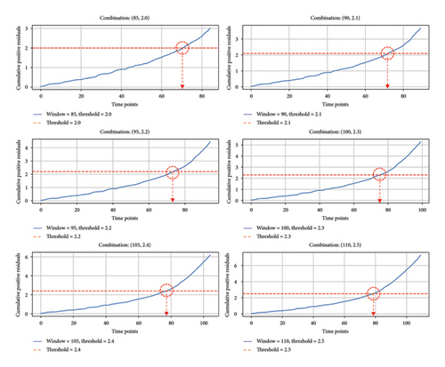
C : [85, 2.0] identifies a significant trend change around Day 70, C : [90, 2.1] around Day 71, C : [95, 2.2] around Day 73, C : [100, 2.3] around Day 75, C : [105, 2.4] around Day 76, and C : [110, 2.5] around Day 78, all occurring prior to the conventional anomaly detection on Day 80. Therefore, the various parameter combinations selected for this simulated seepage risk scenario can achieve early warning effects, indicating that the model has a certain degree of flexibility in parameter selection.

4. Conclusion and Outlook

This paper presents an innovative combined algorithm, AT-LSTM-CUSUM, for predicting dam seepage. The model comprehensively considers five relevant factors: upstream water level, downstream water level, precipitation (processed with de-lagged time series), temperature, and structural aging. By introducing an attention mechanism that dynamically focuses on key factors, the LSTM network is constructed to predict dam seepage. Comparisons with other models reveal that this model achieves good predictive accuracy. In addition, the improved CUSUM algorithm effectively identifies trend changes for early warnings of hidden seepage, although careful consideration of parameter combinations is necessary.

1.
The introduction of an attention mechanism in the LSTM network effectively enhances the model’s predictive accuracy. The AT-LSTM model achieves a goodness of fit of 0.98, with a root mean square error of approximately 0.89 m and a mean absolute error of around 0.62 m. Compared with LSTM, GRU, ARIMA, and Prophet models, the R² value of AT-LSTM improves by 4.6%, 3.3%, 14.3%, and 14.1%, respectively.
2.
The improved CUSUM algorithm effectively identifies trend changes in advance due to the residual accumulation amplification effect and the configuration of the acceptance function, with a certain degree of flexibility in parameter combinations. It can save more than half of the response time compared to commonly used anomaly detection algorithms.
3.
Careful consideration is needed regarding parameter selection for the improved CUSUM model; overly small parameter combinations may lead to excessive sensitivity, while overly large combinations may result in insensitivity.
4.
For dam seepage prediction, more influencing factors could be considered, such as dam construction materials, foundation geology, and seismic activity.
5.
For the improved CUSUM algorithm’s early warning of seepage trend changes, future work could explore integrating specific dam structures, and local hydrological conditions, using cross-validation or statistical methods to find optimal parameter combinations.

Conflicts of Interest

The authors declare no conflicts of interest.

Funding

This research was funded by the National Natural Science Foundation of China (51909204) and Shanxi Natural Science Research Project (20220302121321).

Acknowledgments

The authors acknowledge the National Natural Science Foundation of China (Grant no: 51909204) and Shanxi Natural Science Research Project (20220302121321).

Open Research

Data Availability Statement

The data used to support the findings of this study are available from the corresponding author upon reasonable request.

References

1 Kassahun M. and Matebie M., Seepage Modeling Approaches in the Dam Site and Through the Dam Body: A Review, Arabian Journal of Geosciences. (2024) 17, no. 1.
Google Scholar
2 Zhang J., Yang Z., and Jiang J., An Analysis on Laws of Reservoir Dam Defects and Breaches in China, Scientia Sinica Technologica. (2017) 47, no. 12, 1313–1320, https://doi.org/10.1360/n092016-00295.
10.1360/n092016-00295
Google Scholar
3 Beiranvand B. and Rajaee T., Application of Artificial Intelligence-Based Single and Hybrid Models in Predicting Seepage and Pore Water Pressure of Dams: A State-of-The-Art Review, Advances in Engineering Software. (2022) 173, https://doi.org/10.1016/j.advengsoft.2022.103268.
10.1016/j.advengsoft.2022.103268
Web of Science® Google Scholar
4 Mengfan H. U., Ou B., and Zhang C., Research on Prediction of Earth and Rockfill Dams Based on PSO-BP Model, Water Resources and Power, 89, no. 12, 90–92.
Google Scholar
5 Song J. and Huicheng F. U., Resarch on Prediction of Earth and Rockfill Dams Based on PSO-SVM Model, Water Resources & Hydropower of Northeast China. (2022) 40, no. 11, 40–42.
Google Scholar
6 Nobarinia M., Kalateh F., Nourani V., and Amini A. B., Dam Failure Peak Outflow Prediction Through GEP-SVM Meta Models and Uncertainty Analysis, Water Supply. (2021) 21, no. 7, 3387–3401, https://doi.org/10.2166/ws.2021.100.
10.2166/ws.2021.100
Web of Science® Google Scholar
7 Zhang K., Gu C., Zhu Y., Chen S., Dai B., Li Y., and Shu X., A Novel Seepage Behavior Prediction and Lag Process Identification Method for Concrete Dams Using HGWO-XGBoost Model, IEEE Access. (2021) 9, 23311–23325, https://doi.org/10.1109/access.2021.3056588.
10.1109/access.2021.3056588
Web of Science® Google Scholar
8 Miao X., Shan Y., and Jianwei J. I., Application of PCA-GA-LM Model for Predicting the Seepage of Reservoir Earth-Rockfill Dams, Journal of Shenyang Agricultural University. (2021) 52, no. 3, 377–384.
Google Scholar
9 Khosravi K., Sheikh Khozani Z., and Hatamiafkoueieh J., Prediction of Embankments Dam Break Peak Outflow: A Comparison Between Empirical Equations and Ensemble-Based Machine Learning Algorithms, Natural Hazards. (2023) 118, no. 3, 1989–2018, https://doi.org/10.1007/s11069-023-06060-4.
10.1007/s11069-023-06060-4
Web of Science® Google Scholar
10 Deng Y., Zhang D., Cao Z., and Liu Y., Spatio-Temporal Water Height Prediction for Dam Break Flows Using Deep Learning, Ocean Engineering. (2024) 302, https://doi.org/10.1016/j.oceaneng.2024.117567.
10.1016/j.oceaneng.2024.117567
Web of Science® Google Scholar
11 Chunhui M. A., Hou Y., and Yang J., Seepage Prediction Model of Earth-Rockfill Dams Based on RUN-XGBoost Algorithm, Advances in Science and Technology of Water Resources. (2024) 44, no. 2, 72–78.
Google Scholar
12 Yongtao L. I. U., Zheng D., and Sun X., Time Series Prediction Model of Seepage Flow of an Earth-Rock Dam Based on EEMD-RVM, Advances in Science and Technology of Water Resources. (2021) 41, no. 3, 89–94.
Google Scholar
13 Yan X., Wang X., and Zhao R., Prediction of Earth-Rock Dam Breach Peak Outflow Based on the FFA-GRNN Model, Journal of Changjiang River Scientific Research Institute. (2024) 42, 1–9.
Google Scholar
14 Zhengjie S., Ding Y., and Denghua L., Anomaly Detection of Dam Monitoring Data Based on Prophet-GMM, Yellow River, 142, no. 3, 132–135.
Google Scholar
15 Yue M., Chen X., and Junjie L. I., Seepage Prediction of Concrete Dams Based on CNN-LSTM, Water Resources and Power. (2020) 38, no. 9, 75–78.
Google Scholar
16 Su H., Hu J., and Yang M., Dam Seepage Monitoring Based on Distributed Optical Fiber Temperature System, IEEE Sensors Journal. (2015) 15, no. 1, 9–13, https://doi.org/10.1109/jsen.2014.2335197, 2-s2.0-84910071426.
10.1109/jsen.2014.2335197
Web of Science® Google Scholar
17 Li C., Liu D., Wang M., Wang H., and Xu S., Detection of Outliers in Time Series Power Data Based on Prediction Errors, Energies. (2023) 16, no. 2, https://doi.org/10.3390/en16020582.
10.3390/en16020582
PubMed Web of Science® Google Scholar
18 Malhotra P., Ramakrishnan A., and Anand G., LSTM-Based Encoder-Decoder for Multi-Sensor Anomaly Detection, 2016, https://arxiv.org/abs/1607.00148.
Google Scholar
19 Granjon P., The CuSum Algorithm-A Small Review, 2013, https://hal.science/hal-00914697v1.
Google Scholar
20 Yi F. and Qiu P., An Adaptive CUSUM Chart for Drift Detection, Quality and Reliability Engineering International. (2022) 38, no. 2, 887–894, https://doi.org/10.1002/qre.3020.
10.1002/qre.3020
Web of Science® Google Scholar
21 Chongshi G. U., Lingzhi H. U., and Zhang Q., An Analytic Model for Base Flow of Dam Seepage, Rock and Soil Mechanics. (2005) 7, 1033–1037.
Google Scholar
22 Wang X., Common Diseases and Prevention Measures in Reservoir Engineering, Technology Innovation and Application. (2018) 18, 113–114.
Google Scholar
23 Mukherjee A., Chong Z., and Khoo M., Comparisons of Some Distribution-Free CUSUM and EWMA Schemes and Their Applications in Monitoring Impurity in Mining Process Flotation, Computers & Industrial Engineering. (2019) 137, https://doi.org/10.1016/j.cie.2019.106059, 2-s2.0-85073227301.
10.1016/j.cie.2019.106059
Web of Science® Google Scholar
24 Kinga D. and Adam J. B., A Method for Stochastic Optimization, Proceedings of the International Conference on Learning Representations (ICLR), 2015, 5–6.
Google Scholar
25 Chen S., Gu C., Lin C., Wang Y., and Hariri-Ardebili M. A., Prediction, Monitoring, and Interpretation of Dam Leakage Flow Via Adaptative Kernel Extreme Learning Machine, Measurement. (2020) 166, https://doi.org/10.1016/j.measurement.2020.108161.
10.1016/j.measurement.2020.108161
Web of Science® Google Scholar
26 Alsafadi K., Bi S., Bashir B. et al., High-Resolution Precipitation Modeling in Complex Terrains Using Hybrid Interpolation Techniques: Incorporating Physiographic and MODIS Cloud Cover Influences, Remote Sensing. (2023) 15, no. 9, https://doi.org/10.3390/rs15092435.
10.3390/rs15092435
Web of Science® Google Scholar

All articles

AT-LSTM-CUSUM Digital Intelligent Model for Seepage Safety Prediction of Concrete Dam

Abstract

1. Introduction