In the realm of structural health monitoring (SHM) of bridge structures, the accurate reconstruction of girder-end displacement (GED) is crucial for identifying potential structural damage and ensuring the monitoring system’s reliability. A novel fine-grained spatial (FGS) attention mechanism, combined with efficient channel attention (ECA), has been proposed to effectively utilize multisource monitoring data. This hybrid attention mechanism has been integrated into an arithmetic optimization algorithm–bidirectional long short-term memory (AOA–BiLSTM) framework for reconstructing GED using non-GED data, including deflection, temperature, strain, and traffic data. Data are organized into a two-dimensional array based on sensor types and spatial locations to capture interchannel and intrachannel correlations. ECA captures local correlations among different sensor types, while the proposed FGS enhances model interpretability by focusing on local dependencies within each sensor type. Huber loss is employed for robust performance, and AOA techniques are used for efficient hyperparameter optimization. Validation with real-world data from a cable-stayed bridge demonstrates the necessity and efficacy of considering multidimensional information correlations in response reconstruction for SHM applications. This work lays a theoretical foundation for improving safety assessments, anomaly detection, data recovery, and virtual sensing in bridge structures.

1. Introduction

With the rapid development of modern transportation infrastructure and the gradual aging of bridges constructed in earlier periods, growing attention has been drawn to the safety concerns related to in-service bridges [1–3]. The catastrophic human casualties and substantial economic losses associated with bridge collapse incidents have underscored the critical need for ensuring the operational safety of bridges [4–6]. As a result, structural health monitoring (SHM) systems have been widely implemented to safeguard this essential infrastructure [7–11]. However, due to a range of potential factors such as sensor aging, malfunctions, or random interference, SHM systems inevitably encounter data loss or anomalies (such as bias, outliers, drifting, or noise) in daily operations, consequently hindering the assessment of the structure’s health condition [12]. Therefore, accurate reconstruction of structural responses is of significant importance in the case of sensor or monitoring system faults. It can provide a consistent reference framework for assessing the bridge’s performance and recovering missing data, thereby ensuring the monitoring system’s continuity [13]. Regarding static responses, previous studies have shown that girder-end displacement (GED) monitoring data can illustrate how structures respond to environmental factors and traffic loads, making them one of the most crucial indicators of safety performance [14]. Therefore, the emphasis of this study lies in the real-time reconstruction of GED monitoring data using other types of information.

Structural response reconstruction methods mainly encompass two categories: model-based approaches and data-driven methods. Model-based techniques generally necessitate an understanding of structural characteristics, emphasizing the relationship between external forces and structural deformations [15, 16]. For example, Zhang et al. [17] introduced a method that combines the inverse finite element method (FEM) formulation with the strain-gradient theory to create a nonlinear shape-sensing model for the Euler–Bernoulli beam. In this approach, nonuniform rational B-spline basis functions serve as shape functions to reconstruct the displacements. Although some methods have achieved satisfactory reconstruction results, they largely depend on the accuracy of the FEM [18–21]. These approaches improve prediction accuracy by taking into account material wear and the development process of structural damage. Nonetheless, obstacles and uncertainties arise from the complex mechanisms ruling bridge structural systems, including simplified concrete constitutive theories, unclear degradation processes, and performance disparities among various bridge designs, resulting in application limitations across different bridges [22].

Bridge responses are influenced by multiple factors, including material properties, external loads, weather conditions, and structural aging. It is notably challenging to model the intricate relations among these factors accurately based on physics and mechanics theory alone. Although the influence of these factors on structural responses is not well understood now, the complex mapping relationships between different structural responses can be learned and captured through data-driven approaches [23]. In the SHM system of bridges, there exists not only a degree of association among different types of sensors but also significant spatial correlation among sensor locations. Therefore, the correlation and complementarity among these sensors are expected to improve the performance of response reconstruction, anomaly detection, or virtual sensing by fully leveraging the value of mutual information among multitype sensors, which is possible, to reduce the need for costly or challenging physical measurements [24]. In recent years, this type of model has gained increasing attention to promote the development of SHM. For example, Zhang et al. [25] proposed a multivariate Bayesian dynamic regression method for reconstructing missing SHM data, demonstrating good computational efficiency and accuracy. Principal component analysis and probabilistic principal component analysis have also been employed to extract time-related correlations from various dimensions for the reconstruction of missing data [26]. Additionally, compressed sensing techniques [27, 28] and sparse representation of low-rank data [29] have been successfully applied to the reconstruction of randomly missing acceleration and velocity signals. However, for more complex, large-scale, long-term continuous response reconstruction, traditional data-driven methods may face limitations and performance degradation.

In recent years, deep learning has attracted widespread attention from researchers in the SHM field. Thanks to the powerful nonlinear approximation ability and model generalization performance of deep neural networks, capturing the complex mapping relationships between multitype structural responses has become possible. Jeong et al. [30] proposed a data-driven bidirectional recurrent neural network for sensor data reconstruction, taking into account the spatiotemporal correlations between measured data. Lei et al. [31] proposed a deep convolutional generative adversarial network to reconstruct lost data, utilizing a generator to extract features and reconstruct signals, and a discriminator to improve accuracy. Lu et al. [32] proposed a method for reconstructing structural acceleration responses based on a bidirectional long short-term memory (BiLSTM) network, which explores the complex spatiotemporal correlations between measured data. Wang et al. [33] established a regression model based on long short-term memory (LSTM) to explore the relationship between environmental temperature and the thermally induced low-frequency components in the GED and achieved a reconstruction accuracy for the missing GED data within 10%. Chen [34] proposed a deep learning and autoregressive model with an attention mechanism framework, where a soft attention layer is integrated into the framework following the bidirectional gated recurrent unit layers, serving to eliminate redundant information from multiple sensors. Their results indicate that the response reconstruction performance of the proposed framework surpasses the one-dimensional convolutional neural networks (1D-CNNs) and the hybrid deep learning and autoregressive models.

The aforementioned studies mainly focus on reconstructing structural responses using other types of structural responses, which inevitably neglect the influence of environmental and operational conditions, e.g., temperature and traffic loading. It has been reported that fusing multisource data offers a more comprehensive and effective information base for reconstruction tasks [35]. Taking into account the feature correlation across different types of sensors (e.g., temperature and displacement) as well as the spatial correlation among sensor locations is expected to enhance response reconstruction accuracy [36]. Existing structural response reconstruction techniques predominantly rely on the same type of sensors and often neglect the relationships between different types of sensors. Notably, there is limited research that considers the interdependencies among different types of sensors. For instance, data fusion methods based on LSTM have been employed to reconstruct bridge structures’ deformations using strain and acceleration data [37, 38], without accounting for the intricate correlations between structural responses and environmental conditions. In current practices, data from diverse sensor types, such as GED, deflection, temperature, or strain, are typically integrated as input with only channel attention mechanisms employed to capture dependencies among them [39]. However, this approach has two primary shortcomings. First, it results in a homogenized weighting strategy across all sensor types, thereby neglecting the spatial correlations within each type of sensor. Secondly, conventional attention mechanisms necessitate pooling operations across different dimensions, which merge data from various sensor types, thereby diminishing the model’s sensitivity toward specific physical phenomena. Additionally, hyperparameter selection in deep learning models poses a challenge and current methodologies largely depend on empirical manual settings, which can compromise the accuracy of response reconstruction [40–43]. This issue becomes especially pronounced for SHM of bridges where one-dimensional time series data are measured from each sensor, making it difficult to apply spatial attention mechanisms that are popular in other domains.

To address the aforementioned challenges, this paper introduces a novel fine-grained spatial (FGS) attention mechanism combined with efficient channel attention (ECA) to enhance deep learning’s ability to analyze physical measurements from bridges. This study focuses on reconstructing bridge GED using multisource data such as deflection, temperature, strain, and traffic information. One of the key contributions of this paper is the formulation of input data into two-dimensional arrays based on sensor type and spatial location, enabling the model to capture both sensor type and temporal correlations concurrently. The ECA–FGS attention mechanism is employed to enhance these correlations. The ECA component captures the interrelations among different types of local sensors, while the FGS mechanism prevents the mixing of different physical quantities and enhances model interpretability by focusing specifically on the spatial correlations of each sensor type. To further enhance the model’s robustness against outliers, the Huber loss function is utilized, and the arithmetic optimization algorithm (AOA) is employed for optimizing hyperparameters related to Huber loss and hidden units in the BiLSTM architecture.

2. Methodology

In this study, a BiLSTM [44] is employed for GED reconstruction using non-GED data. The BiLSTM, composed of two LSTM networks, processes input sequences in both forward (start to end) and backward (end to start) directions, integrating past-to-future and future-to-past information flows. To optimize multisource data integration in bridge monitoring, we developed a novel attention mechanism for the BiLSTM, enabling the capture of multilevel information weights.

2.1. BiLSTM Network

The LSTM framework features three pivotal gates: the input gate (regulating new information intake), the forget gate (overseeing the discarding of outdated data), and the output gate (dictating information relay to subsequent network layers). This design equips LSTM to adeptly handle extended dependencies in sequences, offering a marked improvement over standard RNNs [45]. The BiLSTM [46] mirrors the LSTM but processes the input sequence bidirectionally. BiLSTM encompasses dual opposite-direction hidden units, managing sequences from past to future and vice versa. Its final prediction stems from the concatenation or summation of both hidden states, with h_t encapsulating the forward hidden state

and backward hidden state

()

where ⊕ denotes the concatenation operation.

2.2. ECA–FGS Attention Mechanism

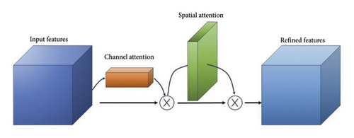
Attention mechanisms enable a model to focus selectively on essential features, assigning varying levels of importance to different components [47]. This is crucial for our task, where the input for each time step is structured as a matrix of dimension C × S, where C represents the number of channels (in this study, the same type of sensors are grouped into one channel) and S denotes the number of sensors in each channel. Please note that the number of sensors for each channel has to be the same due to the matrix structure of the input. Given the dual-dimensional nature of the input (channel and spatial), a specialized attention mechanism is designed to capture both interchannel and intrachannel (spatial) correlations to improve response reconstruction (see Figure 1).

Details are in the caption following the image — **Figure 1**
Open in figure viewer PowerPoint

The framework of attention modules combines both spatial and channel attentiveness.

2.2.1. ECA Mechanism

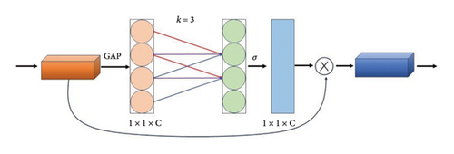
While the convolutional block attention module (CBAM) [48] commonly used in computer vision effectively combines channel and spatial attention, it is less suited for monitoring physical quantities in bridges. CBAM’s reliance on global average and max pooling to extract global statistical characteristics can introduce noise and redundant information into SHM time series data, particularly when the channel scale is small, potentially leading to overfitting. Additionally, while CBAM excels at capturing broad channel dependencies, it struggles with the local dependencies crucial for monitoring bridge data. In contrast, the ECA mechanism, which utilizes 1D convolution along the channel axis [49], aligns more closely with the intrinsic characteristics of bridge data. Figure 2 illustrates the architecture of the employed ECA integrated into the BiLSTM network in this paper.

As shown in Figure 2, ECA first performs global average pooling to transform the feature map and then employs a one-dimensional convolution operation with a kernel size of k, followed by a sigmoid activation function, to obtain the weights ω for each channel:

()

where C1D represents 1D convolution with a kernel size of k. The number of channels C and the 1D convolution kernel size k control the coverage range of cross-channel information interaction, and a proportional relationship exists between them. Furthermore, considering that the channel number C is typically set as a power of 2, a nonlinear mapping relationship can be established as follows:

()

where parameters γ and b are assigned as 2 and 1. Given the channel number C, the kernel size k can be adaptively determined with

()

where ||_odd is the nearest odd number. In this paper, we set C = 4, corresponding to four types of monitoring data: deflection, temperature, strain, and traffic information. Consequently, k is evaluated as 3 based on the above equation.

The original feature map F with size C × S is channel-weighted by the ECA mechanism, resulting in

()

where M_c represents the operation that generates channel-wise weights for the original feature map F based on the ECA mechanism and ⊗ indicates element-wise multiplication. Conventional spatial attention mechanisms, such as the CBAM, generally operate over two spatial dimensions. This is different from the specific application on SHM data of bridge structures, which necessitates attention to be focused solely on dependencies among sensors of the same type, i.e., a one-dimensional spatial correlation within each channel (sensor category).

2.2.2. The Proposed FGS Attention Mechanism

To address the issue of traditional spatial attention mechanisms which mix data from different sensor types such as temperature and deflection through cross-channel pooling [48], we propose the ECA–FGS attention module, combining a novel FGS attention mechanism with ECA. One of the FGS’s attributes is its deliberate avoidance of pooling operations that could intermingle data from different sensor types. To further preserve the integrity of each sensor type while capturing local spatial dependencies, we propose a specialized mapping function defined as

()

In the above mapping function, the domain encapsulates the combined feature space of different sensor types (represented by the channel dimension C) and their respective spatial dimension S. Each channel in the dimension C corresponds to a distinct sensor type, such as temperature, deflection, and, GED. The transformation is carefully architected to yield an output feature space of dimension C × S^′, where S^′ captures the nuanced spatial relationships while giving due attention to local spatial dependencies specific to each sensor. The introduction of this mapping effectively prevents the mixing of different sensor types, thereby enhancing the model’s interpretability. To implement this mapping, FGS employs a specialized 1 × n convolution operation on the feature map F^′ of ECA output:

()

where f_1×n denotes a 1 × n convolution operation,

is the attention weight matrix, and h_t is the hidden state at time t. Padding is applied to ensure that the output feature map retains the original spatial dimensions, which is particularly important in the context of SHM for bridges, where the dimensionality of the sensor data is relatively low. Preserving the spatial dimensions of the input and output data allows us to capture edge information effectively, thereby enhancing the model’s interpretability and performance.

The 1D convolution kernel size n is determined based on the following formula:

()

where [ · ] denotes the ceiling function, which rounds a number up to the nearest integer, and e is the base of the natural logarithm. The initial search space for hyperparameters in the AOA was determined based on the complexity of the data and the authors’ empirical experience. The chosen ranges encompass the optimal values, ensuring that expanding the search space would not affect the final optimized results but could slow down convergence. By limiting the search to this defined range, the optimization process accelerates without compromising accuracy [49].

The attention score is then obtained by the following equation:

()

where the subscript i represents the ith sensor of the specific type. Note that we utilize the sigmoid activation function instead of softmax, which is motivated by our anticipation that multiple variables will contribute meaningfully to the prediction process. This convolutional configuration ensures the operation is confined to the sensor dimension within the same channel (sensor type), allowing for capturing local dependencies among sensors of the same type without contaminating type-specific information distilled by ECA.

The final feature map F^″ is then obtained by element-wise multiplication with the output F^′ from ECA:

()

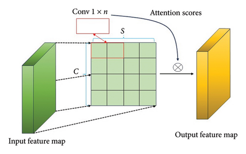
In this way, the ECA–FGS module offers dual advantages: It bolsters the model’s interpretability by preventing the information mixture of different sensor types and enhances performance by effectively capturing local spatial dependencies. Figure 3 shows the structure of the FGS attention mechanism. Given that the spatial dimension of the sensors S = 4 in this paper, the value of n = 2 is derived based on the proposed equation (14), corresponding to the 1D convolution kernel size in Figure 3. The kernel size n impacts the model’s feature extraction: Larger n values capture broader patterns, while smaller ones focus on local details. A careful balance is needed, as large kernels may overlook fine details but aid generalization, whereas small kernels might overfit. Typically, the choice of kernel size is informed by empirical evidence and best practices, which is the purpose of equation (14) to balance granularity with generalization.

2.3. Huber Loss Function

The Huber loss [50], also known as the smooth mean absolute error (MAE), is a loss function used in robust regression, particularly in the presence of outliers. It is less sensitive to outliers in data than the squared error loss. Mathematically, the Huber loss is defined as

()

where a is the difference between the predicted and actual values. The choice of δ determines the point at which the loss transitions from a quadratic to a linear function. If δ is set to a high value, the Huber loss will act similarly to the mean squared error, while if it is set to a low value, it will act similarly to the MAE.

The proposed AOA–BiLSTM and ECA–FGS network is trained using the Adam optimizer, with a maximum of 30 epochs and an initial learning rate of 0.01. A piecewise schedule is employed to reduce the learning rate by 0.1 every 20 epochs. Table 1 details the AOA–BiLSTM and ECA–FGS model architecture, whose framework is shown in Figure 4. The proposed framework integrates several key components to enhance the accuracy of the reconstructed GED. BiLSTM serves as the core sequential model, while AOA optimizes its hyperparameters to ensure the model’s performance. ECA is employed to capture local channel-wise dependencies between different types of sensor data (e.g., temperature, strain, and deflection), while the proposed FGS attention mechanism focuses on refining spatial correlations within each sensor type.

Table 1. Structures of the proposed AOA–BiLSTM and ECA–FGS model.

Block	Layer	Number/size/stride of kernels or number of neurons
Input	Sequence input layer	Size: [4, 4]

Preprocessing	Sequence folding layer	—
Preprocessing	ReLU layer	—

ECA attention	Average pooling layer	Size: [1, 4] for the dimension S
	Convolutional layer	1 kernel of size [3, 1] with padding
	Sigmoid layer	—
	Multiplication layer	—

FGS attention	Convolutional layer	1 kernel of size [1, 2] with padding
	Sigmoid layer	—
	Multiplication layer	—

Sequence learning	Sequence unfolding layer	—
	Flatten layer
	BiLSTM layer	Neurons number determined using AOA

Reconstruction	Huber loss layer	Hyperparameter δ determined using AOA

3. Hyperparameter Optimization and Reconstruction Error Metrics

In the presented model, two pivotal hyperparameters are present which need careful tuning: the number of hidden units u in the BiLSTM and the transition point δ in the Huber loss function. Hyperparameter optimization, a complex nonconvex problem, challenges traditional methods like grid search due to their computational intensity and exhaustive nature, making them impractical for large datasets. Random search and gradient-based methods often fail to find optimal parameters or get trapped in local minima. Similarly, genetic algorithms and particle swarm optimization are slow and prone to suboptimal outcomes. Therefore, this paper utilizes the AOA, whose distinctive exploration and exploitation mechanisms have proven to yield superior performance in nonconvex optimization problems [51].

3.1. AOA

In AOA developed by Abualigah et al. [51], the multiplication and division operations enhance the global dispersion of position updates, while addition and subtraction operations improve the local precision of these updates. The algorithm is characterized by its rapid convergence and high accuracy, which consists of three steps:

1.
The candidate solution is defined as
()
where n represents the number of initial solutions which is set to 20 in this study and m denotes the number of hyperparameters. Here, m = 2, indicating that there are two hyperparameters to optimize, i.e., the number of hidden units u and the transition point δ.
2.
After the initialization step, the math optimizer accelerated (MOA) is computed for exploration purposes, which is derived from
()
where C_iter represents the current iteration and C_iter ∈ (1, M_iter). Max and Min indicate the maximum and minimum values of the acceleration function, respectively. MOA(C_iter) denotes the function value during the tth iteration, which is calculated using the following equation:
()
where C_iter signifies the current iteration, y_i,j(C_iter + 1) denotes the jth position of the ith solution in the subsequent iteration, and best(y_j) is the jth position in the optimal iteration. ε is a small integer number used to prevent division by zero, while ub_j and lb_j, respectively, represent the upper and lower bounds of the jth position. r₂ is a random number in the range of [0,1], and μ is set to 0.5 in this study based on the recommendation [51]. MOP(C_iter) denotes the function value of the math optimizer probability (MOP), which is defined as
()
where M_iter stands for the maximum iterations and α is a sensitive parameter defining the precision of the exploitation process during iterations. In this study, α is set to 5.
3.
Exploitation:
()
To maintain equilibrium between exploration and exploitation, a random number, r₃, in the range of [0,1] is used as a transition criterion. When r₃ > MOA, the candidate solution attempts to diverge from the approximate optimal solution, signifying the algorithm is in the exploration phase. Otherwise, it shifts to exploitation, focusing on refining the solutions in the neighborhood of the current best solution. In this paper, the search space for hyperparameters is set as u ∈ [1, 30] for the number of hidden units and δ ∈ [0.01, 1] for the Huber loss hyperparameter.

3.2. Evaluation Metrics for Response Reconstruction

In this research, we utilize the root mean squared error (RMSE), MAE, average relative percentage error (ARPE), and R-squared score R² as evaluation metrics to evaluate the reconstruction accuracy of bridge response. The mathematical representations of these metrics are as follows:

()

In the above equations, n represents the sample size and x_t and are the monitored and reconstructed data, respectively. A lower MSE, MAE, and ARPE indicate higher reconstruction accuracy, while an R² score closer to 1 suggests a higher fidelity in the reconstructed values to the observed data.

3.3. Visualization for Reconstruction Error

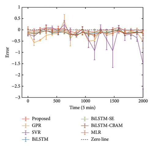
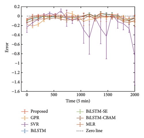
To offer an intuitive representation of the reconstruction precision, we employ visualization techniques, specifically the error bar plot. The error e_i at each time instant denotes the misfit between measured and reconstructed values. Given that the original dataset consists of 2000 data points, a windowing approach is employed to obtain a smooth and stable representation of the errors over time. The errors are divided into nonoverlapping windows with a constant length of 100. Then, within each window, the sample mean and sample standard deviation of the errors are computed. The error bars represent one standard deviation from the mean error within each window. The length of the error bars signifies the level of uncertainty or variability in the errors for that particular window and method.

4. Application to an Existing Bridge

4.1. Overview of the Bridge

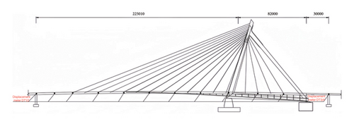
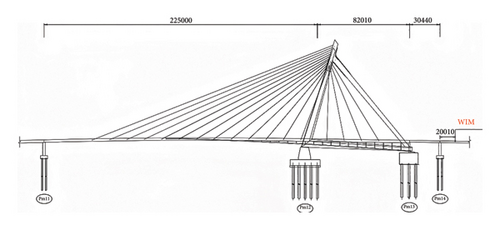
Located in downtown Ningbo, China, the Ningbo Bund Bridge is an asymmetrical cable-stayed structure with a single tower and four cable planes. It features a main span of 225 m and two side spans of 82 and 30 m, totaling 337 m in length. The main girder consists of separate steel box girders connected by transverse girders (for further details, see reference [52]). The Bund Bridge is shown in Figure 5.

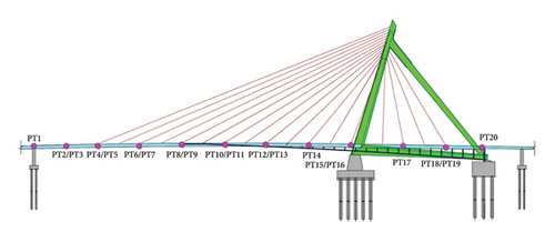
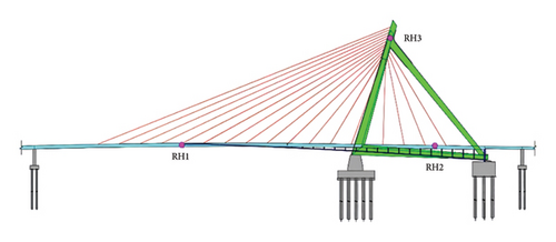
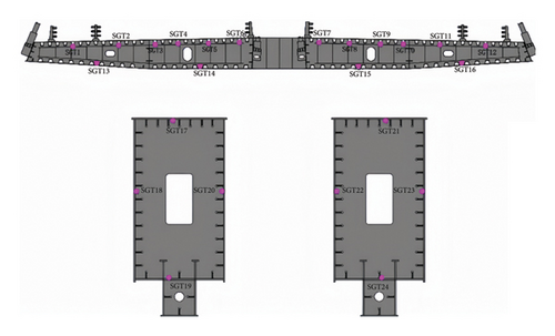
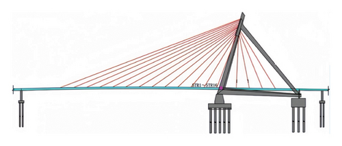
The comprehensive SHM system of the Bund Bridge includes various sensors to monitor key structural and environmental parameters. These sensors measure GED, girder deflection, strain, vehicle weight, and temperature. GED is measured using resistive displacement sensors with an accuracy of 0.01 mm, mounted on embedded steel plates at the side piers (Figure 6(a)). Girder deflections are also recorded by resistive displacement sensors positioned along the main span with a 1-Hz sampling frequency (Figure 6(b)). Environmental temperature is measured with sensors RH1–RH3 (Figure 6(c)); structural temperatures are monitored with SGT1–SGT16 on the girder (Figure 6(d)) and SGT17–SGT24 on the tower (Figure 6(e)). Strain is monitored by resistive strain gauges with an accuracy of 0.25%, installed at the girder-tower connection (STR1–STR16, Figures 6(f) and 6(g)). Vehicle weights are measured by a weigh-in-motion (WIM) system located at the bridge entrance (Figure 6(h)).

To ensure accurate reconstruction of GED and consider the effects of temperature, vehicle weight, strain, and deflection, these measured data are integrated into the AOA–BiLSTM model with ECA–FGS attention mechanisms.

4.2. Data Preparation

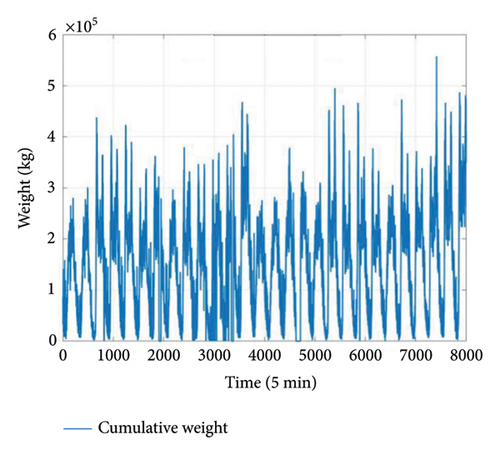
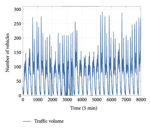
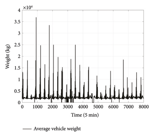
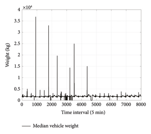
As raw measurement data are disturbed by many transient and irrelevant factors, the measured GED data are averaged at every 5-min window to reduce noise and obtain smoother GED value. Similarly, the input data for reconstruction, including strain, temperature, and girder deflection, are also averaged at every 5-min window. The length of 5-min window used in this study allows for smoothing the raw measurements to remove random fluctuations, meanwhile still possessing the short-term variations of measured information. As for the traffic weights measured by WIM, 4 different traffic metrics are defined to provide a comprehensive profile of traffic load on the bridge within every 5-min window, i.e., cumulative vehicle weights in every 5-min window, average vehicle weights, median vehicle weights, and traffic volume (number of vehicles).

The 5-min average GED data from April 18, 2020, to May 14, 2020, are used as the target output in this study, including the GED sensors DT2, DT3, and DT4. Following the proposed framework, a 2D input structure is constructed whose rows correspond to types of sensors and columns correspond to specific sensors within each type. Given that four types/channels of data are considered (deflection, temperature, strain, and traffic information), the channel dimension is set to four. To encapsulate a wide range of features within each channel, 4 sensors/metrics are selected for each channel. For deflection data, inputs are PT1, PT6, PT13, and PT15 (Figure 7(a)). Deflections vary across these locations due to differences in structural position, load distribution, and support conditions. For temperature data, the selected sensors are RH1, RH2, RH3 (ambient), and SGT14 (structural) (Figure 7(b)). Ambient sensors show similar readings, while SGT14 exhibits higher variability due to thermal responses in the structure. For strain data, inputs include STR4, STR7, STR9, and STR14 (Figure 7(c)). Strain differences arise from localized stress variations due to bending moments and axial forces at different points. The traffic data comprise cumulative weight, average weight, median weight, and traffic volume (Figure 8). Variations in these metrics reflect nonuniform traffic patterns and vehicle types. Despite the differences in these measurements, they exhibit correlations due to the interconnected nature of the structural behavior under various loads. For instance, deflection and strain are both influenced by vehicle load and traffic volume, and temperature fluctuations can impact strain and deflection through material thermal expansion and contraction.

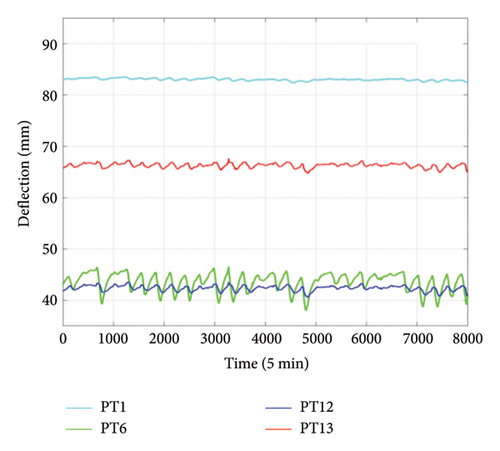
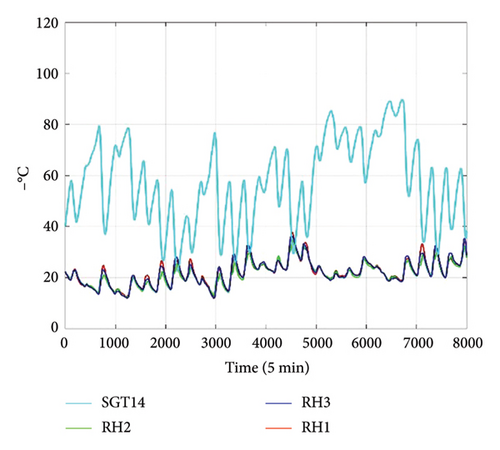
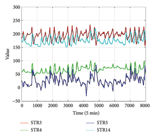
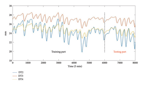
For the target GED data, we consider the first 6000 data points as known information for model training, while the subsequent 2000 data points are utilized to validate the reconstruction performance of the model, as shown in Figure 9. Specifically, a 3D total input with a size of [4, 4, 6000] is utilized for learning the target deflection data.

4.3. Reconstruction Results Based on AOA–BiLSTM and ECA–FGS

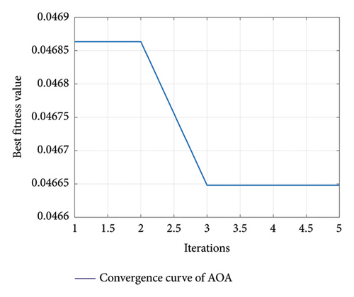
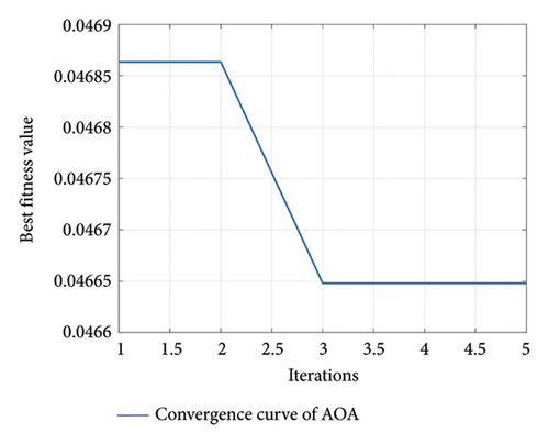
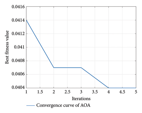
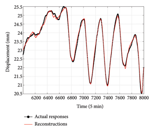
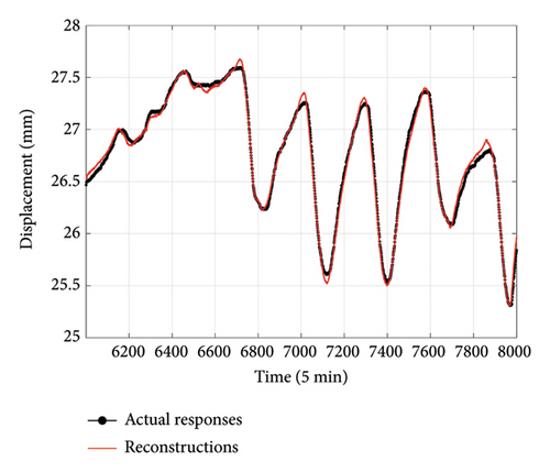
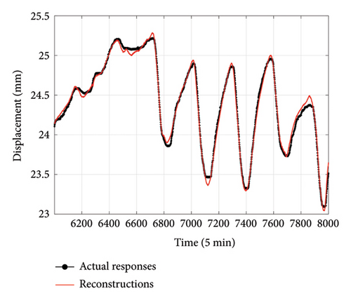
The optimization of the number of hidden units in BiLSTM and the hyperparameter of the Huber loss function is performed using the AOA method presented in Section 3. The optimization results, as shown in Figure 10, indicate rapid convergence after five iterations. The optimized hyperparameter combinations (u, δ) at locations DT2, DT3, and DT4 are (16, 0.05), (21, 0.04), and (18, 0.07), respectively. Then, the proposed AOA–BiLSTM integrated with ECA–FGS attention is trained using the previously discussed input and target data. The GED reconstruction results are illustrated in Figures 11(a), 11(b), and 11(c), corresponding to the sensors DT2, DT3, and DT4, respectively. A good agreement between the reconstructed and the actual responses can be observed, despite some discrepancies existing, especially at the peaks and valleys for DT4. The RMSE, MAE, ARPE, and R² are reported in Tables 2, 3, and 4 for DT2, DT3, and DT4, respectively. All error metrics are relatively small, with an R² very close to 1, indicating excellent reconstruction performance.

Table 2. Comparison of reconstruction results for DT2.

Methods	Proposed	GPR	SVR	BiLSTM	BiLSTM-SE	BiLSTM-CBAM	MLR
RMSE	0.1088	0.3458	0.6103	0.1652	0.1558	0.1673	0.1542
MAE	0.0884	0.2564	0.3510	0.1331	0.1253	0.1392	0.1247
ARPE	0.3751	1.0992	1.5699	0.5621	0.5324	0.5941	0.5336
R²	0.9923	0.9222	0.7575	0.9822	0.9842	0.9818	0.9838

Table 3. Comparison of reconstruction results for DT3.

Methods	Proposed	GPR	SVR	BiLSTM	BiLSTM-SE	BiLSTM-CBAM	MLR
RMSE	0.0443	0.1434	0.3553	0.0551	0.0527	0.0816	0.0512
MAE	0.0348	0.1063	0.2056	0.0437	0.0415	0.0690	0.0394
ARPE	0.1303	0.4029	0.7852	0.1636	0.1552	0.2578	0.1463
R²	0.9939	0.9370	0.6132	0.9907	0.9915	0.9796	0.9910

Table 4. Comparison of reconstruction results for DT4.

Methods	Proposed	GPR	SVR	BiLSTM	BiLSTM-SE	BiLSTM-CBAM	MLR
RMSE	0.0457	0.1463	0.2997	0.0543	0.0514	0.0576	0.0553
MAE	0.0374	0.1170	0.1747	0.0431	0.0411	0.0460	0.0462
ARPE	0.1538	0.4834	0.7313	0.1769	0.1692	0.1893	0.1839
R²	0.9930	0.9280	0.6981	0.9901	0.9911	0.9888	0.9873

4.4. Comparison With Other Methods

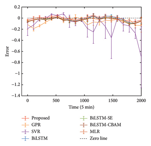
To rigorously evaluate the reconstruction performance of the proposed method, a comparative analysis is conducted to compare the reconstruction results of GED obtained through the proposed model with those derived from Gaussian process regression (GPR) [53], support vector regression (SVR) [54], standard BiLSTM [44] approaches, BiLSTM approaches with squeeze-and-excitation attention mechanism (BiLSTM-SE) [55] for channel attention, and BiLSTM variants that employ CBAM (BiLSTM-CBAM) [48] for channel and spatial attention. Additionally, multiple linear regression (MLR) is included as a baseline, with its fixed-weight characteristic used to validate the effectiveness of the attention mechanism’s dynamic, data-driven weighting, which adapts based on input features in a deep learning framework. The reconstruction outcomes for the six approaches are illustrated in Figures 12(a), 12(b), and 12(c), corresponding to sensors DT2, DT3, and DT4, respectively. It can be observed that the proposed method demonstrates clear advantages in both peak regions and overall alignment. The precision metrics presented in Tables 2, 3, and 4, including MSE, MAE, RPE, and R², further confirm this conclusion, as the proposed method consistently achieves the highest accuracy across all three datasets. Notably, the BiLSTM-CBAM method performs the worst among the BiLSTM-based approaches, likely due to the CBAM confusing different types of monitoring variables. Similarly, MLR performs worse than the proposed method, as its fixed-weight nature limits its ability to capture the complex, dynamic relationships between the input features and the target variable.

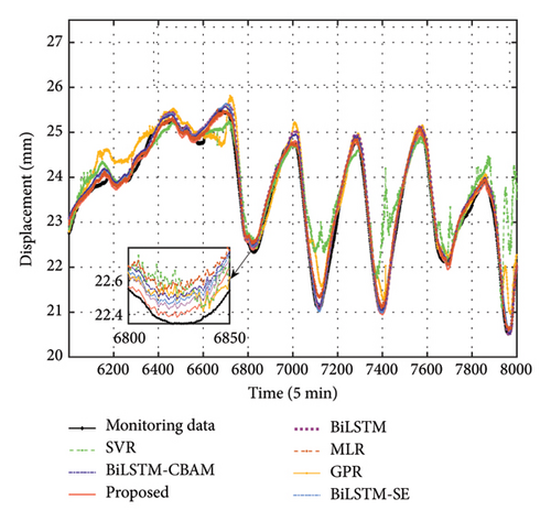
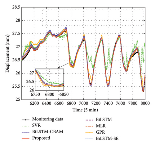
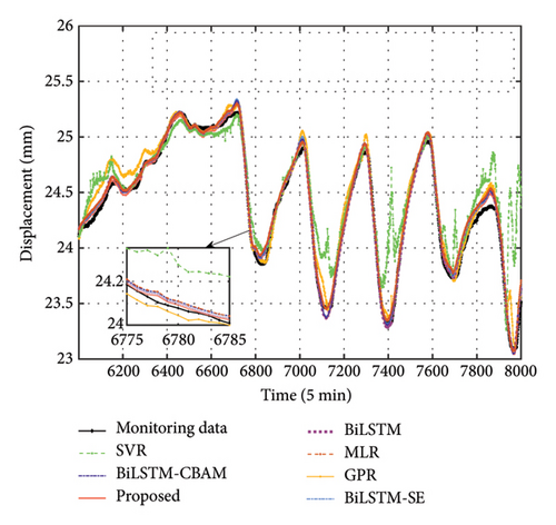
To further quantify the advantages, we compared the MAE, showing that our method improves by an average of 66.94% over GPR, 78.83% over SVR, 22.39% over BiLSTM, 18.20% over BiLSTM-SE, 34.92% over BiLSTM-CBAM, and 19.94% over MLR across three datasets. In anomaly detection, larger reconstruction errors may indicate potential structural anomalies. The robustness and precision of the proposed method provide a clear advantage, making it especially well-suited for identifying such anomalies with greater accuracy and reliability. Subsequently, employing the visualization techniques outlined in Section 3.2, we generate error bars for each of the five different approaches. These results are illustrated in Figures 13(a), 13(b), and 13(c). For this analysis, we adopt a window size w = 100, meaning that the mean and standard deviation of the error are calculated over each set of 100 data points. Upon reviewing the figures, it is clear that our proposed method yields an error closest to zero mean and exhibits the lowest standard deviation, as indicated by the narrow error bars, underscoring its superior stability compared to other methods.

4.5. Anomaly Detection Simulation

In addition to directly reconstructing missing data for data recovery, the proposed method can also be employed for anomaly detection. To demonstrate the anomaly detection capability of the proposed method, a simulation experiment based on DT2 data is conducted. An increasing linear trend is superposed on the original DT2 data within the time range of [1800 2000], as depicted in Figure 14. This simulation represents a scenario where local damage, particularly cracks near the supports, reduces local stiffness and primarily affects the GED [56, 57], while other inputs, such as temperature, deflection, traffic information, and longitudinal stress at mid-span, remain unchanged. This local damage minimally impacts overall deflection but significantly alters the GED. In actual cable-stayed bridges, the correlation between deflection and GED is often weak, as deflection and strain in the main girder are mainly influenced by vertical loads, while end displacement is more sensitive to support conditions. However, deflection is still included as it can slightly improve GED reconstruction accuracy when combined with other monitoring data in a multisource approach. In practice, temperature shows the highest correlation with GED [58], but other inputs provide marginal improvements. Therefore, when the temperature remains stable but GED shows significant changes, anomalies can be more easily identified.

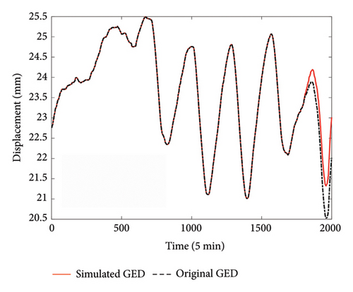
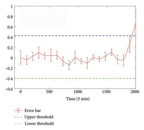
The comparison of simulated GED data and reconstructed response is shown in Figure 15(a). It is seen that a large discrepancy in the superposed increasing trend is present which reflects the potential anomaly. To provide an objective metric for anomaly detection, the error bar plot is employed here to establish the warning threshold. Since the first 1000 samples are known to be normal, their sample statistics of reconstruction errors are utilized to derive the deviation bounds of errors, which includes the following steps: (1) First evaluate the sample mean and standard deviations at each window of length 100 (i.e., 10 windows for 1000 samples); (2) compute the bounds at 10 windows based on three-sigma rule, i.e., the upper and lower values of three standard deviations of mean values; and (3) choose the maximum upper bound value among all 10 windows as the upper threshold, and similarly choose the minimum lower bound value among all 10 windows as the lower threshold. These upper and lower thresholds represent the normal range of reconstruction errors and are used to detect the abnormal state when the error exceeds them. The error bar chart is depicted in Figure 15(b). A noticeably large standard deviation at the 20th window (corresponding to the 1800th to 2000th data points given a window length of 100) is observed, whose error bar surpasses the upper threshold line, successfully detecting the simulated anomaly. Note that this section serves as a primitive study for anomaly detection and is included here for demonstration, and experimental studies on laboratory models or field structures are needed to further validate its efficacy on anomaly detection.

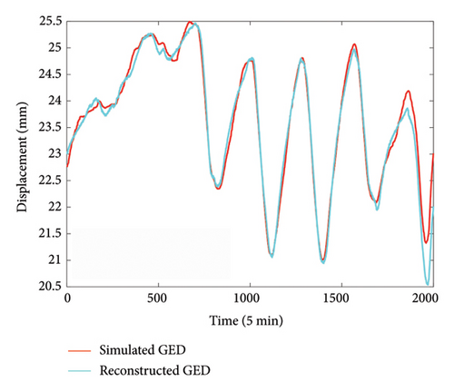
In practical applications, sensor measurement characteristics and noise may change over time. The adaptability of the proposed method to varying sensor configurations can be achieved considering the high flexibility of the proposed attention mechanism and employing regular updates of the model, for example: (1) the attention mechanism adaptively assigns lower weights to noisy data, capturing more valuable information and reducing the impact of noise; (2) the implementation of the Huber loss function within the model further enhances its robustness to noise; and (3) regular reevaluation and updates of the model ensure its alignment with the current state of the sensors. It is noteworthy that significant data drift, as illustrated in Figure 15, may indicate anomalies in the sensors or the structure. Interestingly, these features enable the use of models trained on historical monitoring data, such as data from 5 years ago, to reconstruct target responses based on current sensor readings, enabling direct estimation of the extent of GED growth under long-term influences.

5. Conclusions

In this study, we introduced an innovative deep learning framework for the reconstruction of GED from non-GED sensor data. To address the limitations of conventional methods in utilizing multisource data, we employed a two-dimensional data representation based on sensor types and spatial layouts. This structure enabled the simultaneous exploitation of intersensor-type correlations and spatial dependencies within each sensor type. A novel attention mechanism, termed FGS attention, was proposed to capture these intricate dependencies more effectively. The FGS mechanism enhances the model’s interpretability by focusing on local spatial dependencies within individual sensor types, avoiding the conflation of different physical quantities. This mechanism was combined with ECA, which focuses on local intersensor-type correlations. The hybrid attention mechanism was integrated into a BiLSTM architecture for GED reconstruction using non-GED data, including deflection, temperature, strain, and traffic data. The framework employs Huber loss for robust performance and leverages an AOA for efficient hyperparameter optimization.

Validation studies are conducted to reconstruct the measured GED data at three locations using non-GED information including girder deflection, temperature, strain, and traffic conditions from the SHM system of a cable-stayed bridge. The experimental results show that, under the same configuration parameters, our ECA–FGS-equipped AOA–BiLSTM framework significantly outperforms standard BiLSTM approaches, BiLSTM with only SE for channel attention, and BiLSTM variants that employ CBAM for channel and spatial attention. Comparative analyses with traditional machine learning methods such as GPR and SVR further confirm the robustness and superiority of our approach in handling multisource bridge data. For the cable-stayed bridge in this paper, the MAE of reconstruction results is even less than 0.1 mm. Moreover, based on the numerical study, it is possible to detect structural anomalies utilizing error bar charts of the reconstructed GED.

While the proposed method has been validated on a specific cable-stayed bridge, its data-driven nature enhances its versatility, making it suitable for other bridge types (e.g., suspension or arch bridges) and even other civil structures, provided the sensors capture relevant physical quantities. The findings underscore the necessity and effectiveness of considering sensor data correlations from multiple perspectives in the context of bridge health monitoring and response reconstruction. The theoretical contributions of our work lay a strong foundation for applications in bridge structural safety assessment, anomaly detection, data recovery, and virtual sensing.

Conflicts of Interest

The authors declare no conflicts of interest.

Funding

This work was supported by the National Natural Science Foundation of China (Grant Nos. 52208199 and 52378187), the Shanghai Science and Technology Cooperation Project of QiZhi Research Institute (Grant No. SQZ202310), and the Fundamental Research Funds for the Central Universities.

Acknowledgments

We would like to thank our funding agency for their generous support of this project. This work was supported by the National Natural Science Foundation of China (Grant Nos. 52208199 and 52378187), the Shanghai Science and Technology Cooperation Project of QiZhi Research Institute (Grant No. SQZ202310), and the Fundamental Research Funds for the Central Universities. No artificial intelligence tools were employed in the preparation of this manuscript. The authors take full responsibility for independently developing and reviewing all contents.

Open Research

Data Availability Statement

The data that support the findings of this study are available from the corresponding author upon reasonable request.

References

1 Ghiasi A., Ng C.-T., and Sheikh A. H., Damage Detection of In-Service Steel Railway Bridges Using a Fine K-Nearest Neighbor Machine Learning Classifier, Structures. (2022) 45, 1920–1935, https://doi.org/10.1016/j.istruc.2022.10.019.
10.1016/j.istruc.2022.10.019
Web of Science® Google Scholar
2 Capogna M., Salvatore W., Renzi E., and Tamasi G., Guidelines for the Classification and Management of Risk, for the Evaluation of Safety and for the Monitoring of Existing Bridges, Procedia Structural Integrity. (2023) 44, 705–712, https://doi.org/10.1016/j.prostr.2023.01.092.
10.1016/j.prostr.2023.01.092
Google Scholar
3 Payawal J. M. G. and Kim D. K., A Review on the Latest Advancements and Innovation Trends in Vibration-Based Structural Health Monitoring (SHM) Techniques for Improved Maintenance of Steel Slit Damper (SSD), IEEE Access. (2024) 12, 44383–44400, https://doi.org/10.1109/access.2024.3381625.
10.1109/ACCESS.2024.3381625
Web of Science® Google Scholar
4 Khoeri H., Isvara W., Widjajakusuma J., Natasa F., and Sofiana D., Static Load Testing of PCI-Bridges for Assessing Functional Suitability and its Comparison with Dynamic Testing, Reka Buana: Jurnal Ilmiah Teknik Sipil dan Teknik Kimia. (2024) 9, no. 1, 55–69, https://doi.org/10.33366/rekabuana.v9i1.5655.
10.33366/rekabuana.v9i1.5655
Google Scholar
5 Rizzo P. and Enshaeian A., Challenges in Bridge Health Monitoring: A Review, Sensors. (2021) 21, no. 13, https://doi.org/10.3390/s21134336.
10.3390/s21134336
Web of Science® Google Scholar
6 Wang G. and Ke J., Literature Review on the Structural Health Monitoring (SHM) of Sustainable Civil Infrastructure: An Analysis of Influencing Factors in the Implementation, Buildings. (2024) 14, no. 2, https://doi.org/10.3390/buildings14020402.
10.3390/buildings14020402
Web of Science® Google Scholar
7 Qu G., Song M., Xin G., Shang Z., and Sun L., Time-convolutional Network with Joint Time-Frequency Domain Loss Based on Arithmetic Optimization Algorithm for Dynamic Response Reconstruction, Engineering Structures. (2024) 321, https://doi.org/10.1016/j.engstruct.2024.119001.
10.1016/j.engstruct.2024.119001
Web of Science® Google Scholar
8 Chen R. and Ni Y. Q., A Nonparametric Bayesian Approach for Bridge Reliability Assessment Using Structural Health Monitoring Data, Structural Control and Health Monitoring. (2023) 2023, 1–25, https://doi.org/10.1155/2023/9271433.
10.1155/2023/9271433
CAS Web of Science® Google Scholar
9 Morgese M., Wang C., Taylor T., Etemadi M., and Ansari F., Distributed Detection and Quantification of Cracks in Operating Large Bridges, Journal of Bridge Engineering. (2024) 29, no. 1, https://doi.org/10.1061/jbenf2.beeng-6454.
10.1061/JBENF2.BEENG-6454
Web of Science® Google Scholar
10 Aktan E., Bartoli I., Glišić B., and Rainieri C., Lessons from Bridge Structural Health Monitoring (SHM) and Their Implications for the Development of Cyber-Physical Systems, Infrastructures. (2024) 9, no. 2, https://doi.org/10.3390/infrastructures9020030.
10.3390/infrastructures9020030
Web of Science® Google Scholar
11 Qu G., Xia Y., Sun L., and Xin G., Behavior Expectation-Based Anomaly Detection in Bridge Deflection Using AOA-BiLSTM-TPA: Considering Temperature and Traffic-Induced Temporal Patterns, Structural Control and Health Monitoring. (2024) 2024, no. 1, https://doi.org/10.1155/2024/2337057.
10.1155/2024/2337057
Web of Science® Google Scholar
12 Fan G., He Z., and Li J., Structural Dynamic Response Reconstruction Using Self-Attention Enhanced Generative Adversarial Networks, Engineering Structures. (2023) 276, https://doi.org/10.1016/j.engstruct.2022.115334.
10.1016/j.engstruct.2022.115334
Web of Science® Google Scholar
13 Talebi-Kalaleh M. and Mei Q., Damage Detection in Bridge Structures through Compressed Sensing of Crowdsourced Smartphone Data, Structural Control and Health Monitoring. (2024) 2024, no. 1, https://doi.org/10.1155/2024/5436675.
10.1155/2024/5436675
Web of Science® Google Scholar
14 Liu Qi-yang, Geng J.-wei, Wang Y., Ge Y., and Bao Q., Multi-Parameter Damper Optimization of Cable-Stayed Bridge Considering Energy Dissipation, Journal of Physics: Conference Series. (2023) 2541, no. 1, https://doi.org/10.1088/1742-6596/2541/1/012002.
10.1088/1742-6596/2541/1/012002
Google Scholar
15 Song M., Christensen S., Moaveni B., Brandt A., and Hines E., Joint Parameter-Input Estimation for Virtual Sensing on an Offshore Platform Using Output-Only Measurements, Mechanical Systems and Signal Processing. (2022) 170, https://doi.org/10.1016/j.ymssp.2022.108814.
10.1016/j.ymssp.2022.108814
Web of Science® Google Scholar
16 Bakhshandeh M., Bridge Health Monitoring: A Review, International Journal of Structural and Construction Engineering. (2024) 18, no. 2, 57–70.
Google Scholar
17 Zhao F., Bao H., and Zhang F., Geometrically Nonlinear Deformation Reconstruction of Based on Euler–Bernoulli Beam Theory Using a Nonlinear iFEM Algorithm, Thin-Walled Structures. (2023) 189, https://doi.org/10.1016/j.tws.2023.110884.
10.1016/j.tws.2023.110884
Web of Science® Google Scholar
18 Altunişik A. C., Kalkan E., Okur F. Y., Karahasan O. Ş., and Ozgan K., Finite-element Model Updating and Dynamic Responses of Reconstructed Historical Timber Bridges Using Ambient Vibration Test Results, Journal of Performance of Constructed Facilities. (2020) 34, no. 1, https://doi.org/10.1061/(asce)cf.1943-5509.0001344.
10.1061/(ASCE)CF.1943-5509.0001344
Web of Science® Google Scholar
19 Huang T., Dong T., and Yuan S., A Piecewise Inverse Finite Element Method for Shape Sensing of the Morphing Wing Fishbone, Smart Materials and Structures. (2024) 33, no. 4, https://doi.org/10.1088/1361-665x/ad2c70.
10.1088/1361-665X/ad2c70
Web of Science® Google Scholar
20 Krysko A. V., Kalutsky L. A., and Krysko V. A., Stress-strain State of a Porous Flexible Rectangular FGM Size-dependent Plate Subjected to Different Types of Transverse Loading: Analysis and Numerical Solution Using Several Alternative Methods, Thin-Walled Structures. (2024) 196, https://doi.org/10.1016/j.tws.2023.111512.
10.1016/j.tws.2023.111512
Web of Science® Google Scholar
21 Sánchez-Haro J., Lombillo I., and Capellán G., Modelling Criteria Proposal for Dynamic Analysis of Beam Bridges under Moving Loads Using Fem Models, Structures. (2023) 50, 651–669, https://doi.org/10.1016/j.istruc.2023.02.067.
10.1016/j.istruc.2023.02.067
Web of Science® Google Scholar
22 Zhu J. and Forman J., A Review of Finite Element Models of Ligaments in the Foot and Considerations for Practical Application, Journal of Biomechanical Engineering. (2022) 144, no. 8, https://doi.org/10.1115/1.4053401.
10.1115/1.4053401
Web of Science® Google Scholar
23 Zhao H., Tan C., Obrien E. J., Zhang B., Uddin N., and Guo H., Developing Digital Twins to Characterize Bridge Behavior Using Measurements Taken under Random Traffic, Journal of Bridge Engineering. (2022) 27, no. 1, https://doi.org/10.1061/(asce)be.1943-5592.0001814.
10.1061/(ASCE)BE.1943-5592.0001814
Web of Science® Google Scholar
24 Maes K. and Lombaert G., Validation of Virtual Sensing for the Reconstruction of Stresses in a Railway Bridge Using Field Data of the KW51 Bridge, Mechanical Systems and Signal Processing. (2023) 190, https://doi.org/10.1016/j.ymssp.2023.110142.
10.1016/j.ymssp.2023.110142
Web of Science® Google Scholar
25 Zhang Yi-M., Wang H., Bai Yu, Mao J.-X., and Xu Yi-C., Bayesian Dynamic Regression for Reconstructing Missing Data in Structural Health Monitoring, Structural Health Monitoring. (2022) 21, no. 5, 2097–2115, https://doi.org/10.1177/14759217211053779.
10.1177/14759217211053779
Web of Science® Google Scholar
26 Li L., Liu H., Zhou H., and Zhang C., Missing Data Estimation Method for Time Series Data in Structure Health Monitoring Systems by Probability Principal Component Analysis, Advances in Engineering Software. (2020) 149, https://doi.org/10.1016/j.advengsoft.2020.102901.
10.1016/j.advengsoft.2020.102901
Web of Science® Google Scholar
27 Mascareñas D., Cattaneo A., Theiler J., and Farrar C., Compressed Sensing Techniques for Detecting Damage in Structures, Structural Health Monitoring. (2013) 12, no. 4, 325–338, https://doi.org/10.1177/1475921713486164, 2-s2.0-84879940207.
10.1177/1475921713486164
Web of Science® Google Scholar
28 Peckens C. A. and Lynch J. P., Utilizing the Cochlea as a Bio-Inspired Compressive Sensing Technique, Smart Materials and Structures. (2013) 22, no. 10, https://doi.org/10.1088/0964-1726/22/10/105027, 2-s2.0-84884578229.
10.1088/0964-1726/22/10/105027
Web of Science® Google Scholar
29 Yang Y. and Nagarajaiah S., Harnessing Data Structure for Recovery of Randomly Missing Structural Vibration Responses Time History: Sparse Representation versus Low-Rank Structure, Mechanical Systems and Signal Processing. (2016) 74, 165–182, https://doi.org/10.1016/j.ymssp.2015.11.009, 2-s2.0-84961124884.
10.1016/j.ymssp.2015.11.009
Web of Science® Google Scholar
30 Jeong S., Ferguson M., Hou R., Lynch J. P., Sohn H., and Law K. H., Sensor Data Reconstruction Using Bidirectional Recurrent Neural Network With Application to Bridge Monitoring, Advanced Engineering Informatics. (2019) 42, https://doi.org/10.1016/j.aei.2019.100991.
10.1016/j.aei.2019.100991
Web of Science® Google Scholar
31 Lei X., Sun L., and Xia Ye, Lost Data Reconstruction for Structural Health Monitoring Using Deep Convolutional Generative Adversarial Networks, Structural Health Monitoring. (2021) 20, no. 4, 2069–2087, https://doi.org/10.1177/1475921720959226.
10.1177/1475921720959226
Web of Science® Google Scholar
32 Lu Y., Tang L., Chen C. et al., Reconstruction of Structural Long-Term Acceleration Response Based on BiLSTM Networks, Engineering Structures. (2023) 285, https://doi.org/10.1016/j.engstruct.2023.116000.
10.1016/j.engstruct.2023.116000
Web of Science® Google Scholar
33 Wang Z., Lu X., Zhang W., Fragkoulis V. C., Beer M., and Zhang Y., Deep Learning-Based Reconstruction of Missing Long-Term Girder-End Displacement Data for Suspension Bridge Health Monitoring, Computers & Structures. (2023) 284, https://doi.org/10.1016/j.compstruc.2023.107070.
10.1016/j.compstruc.2023.107070
Web of Science® Google Scholar
34 Chen C., Tang L., Lu Y. et al., Temperature-induced Response Reconstruction Method Based on DL-AR Model and Attention Mechanism, Structures. (2023) 50, 359–372, https://doi.org/10.1016/j.istruc.2023.02.044.
10.1016/j.istruc.2023.02.044
Web of Science® Google Scholar
35 Fu M., Liang Y., Feng Q., Wu B., and Tang G., Research on the Application of Multi-Source Data Analysis for Bridge Safety Monitoring in the Reconstruction and Demolition Process, Buildings. (2022) 12, no. 8, https://doi.org/10.3390/buildings12081195.
10.3390/buildings12081195
Web of Science® Google Scholar
36 Kim S., Park So Y., Shin J., Choi I. R., and Choi S., Deep-learning-based Data Loss Reconstruction for Spatiotemporal Temperature in Piloti Structures: Enhancing Applicability with Limited Datasets, Fire Safety Journal. (2023) 140, https://doi.org/10.1016/j.firesaf.2023.103887.
10.1016/j.firesaf.2023.103887
Web of Science® Google Scholar
37 Duan Da-Y., Wang Z.-C., Sun X.-T., and Xin Yu, A Data Fusion Method for Bridge Displacement Reconstruction Based on LSTM Networks, Smart Structures and Systems. (2022) 29, no. 4.
Web of Science® Google Scholar
38 Zhang Li-K. and Zuo-Cai W., A Multi-Source Data Fusion Method for Bridge Displacement Reconstruction Based on LSTM Neural Network, Journal of Civil & Environmental Engineering. (2022) 44, no. 3, 37–43.
CAS Google Scholar
39 Liao Y., Lin R., Zhang R., and Wu G., Attention-based LSTM (AttLSTM) Neural Network for Seismic Response Modeling of Bridges, Computers & Structures. (2023) 275, https://doi.org/10.1016/j.compstruc.2022.106915.
10.1016/j.compstruc.2022.106915
Web of Science® Google Scholar
40 Papavasileiou P., Koronaki E. D., Pozzetti G. et al., Equation-based and Data-Driven Modeling Strategies for Industrial Coating Processes, Computers in Industry. (2023) 149, https://doi.org/10.1016/j.compind.2023.103938.
10.1016/j.compind.2023.103938
Web of Science® Google Scholar
41 Niu J., Li Z., Zhuo Yi et al., Robust Correlation Mapping of Train-Induced Stresses for High-Speed Railway Bridge Using Convolutional Denoising Autoencoder, Structural Health Monitoring. (2023) 22, no. 2, 832–845, https://doi.org/10.1177/14759217221095191.
10.1177/14759217221095191
Web of Science® Google Scholar
42 Gao S., Zhao W., Wan C., Jiang H., Ding Y., and Xue S., Missing Data Imputation Framework for Bridge Structural Health Monitoring Based on Slim Generative Adversarial Networks, Measurement. (2022) 204, https://doi.org/10.1016/j.measurement.2022.112095.
10.1016/j.measurement.2022.112095
PubMed Web of Science® Google Scholar
43 Rimal Y., Sharma N., and Alsadoon A., The Accuracy of Machine Learning Models Relies on Hyperparameter Tuning: Student Result Classification Using Random Forest, Randomized Search, Grid Search, Bayesian, Genetic, and Optuna Algorithms, Multimedia Tools and Applications. (2024) 83, no. 30, 74349–74364, https://doi.org/10.1007/s11042-024-18426-2.
10.1007/s11042-024-18426-2
Web of Science® Google Scholar
44 Siami-Namini S., Tavakoli N., and Namin A. S., The Performance of LSTM and BiLSTM in Forecasting Time Series, 2019 IEEE International Conference on Big Data (Big Data). (2019) 3285–3292, https://doi.org/10.1109/bigdata47090.2019.9005997.
10.1109/BigData47090.2019.9005997
Google Scholar
45 Staudemeyer R. C. and Morris E. R., Understanding LSTM--a Tutorial into Long Short-Term Memory Recurrent Neural Networks, arXiv preprint arXiv:1909.09586. (2019) .
Google Scholar
46 Yang M. and Wang J., Adaptability of Financial Time Series Prediction Based on BiLSTM, Procedia Computer Science. (2022) 199, 18–25, https://doi.org/10.1016/j.procs.2022.01.003.
10.1016/j.procs.2022.01.003
Google Scholar
47 Vaswani A., Shazeer N., Parmar N. et al., Attention Is All You Need, Advances in Neural Information Processing Systems. (2017) .
Google Scholar
48 Woo S.n et al., Cbam: Convolutional Block Attention Module, Proceedings of the European Conference on Computer Vision (ECCV), June 2018.
Google Scholar
49 Khatibinia M. and Yazdani H., Accelerated Multi-Gravitational Search Algorithm for Size Optimization of Truss Structures, Swarm and Evolutionary Computation. (2018) 38, 109–119, https://doi.org/10.1016/j.swevo.2017.07.001, 2-s2.0-85021697672.
10.1016/j.swevo.2017.07.001
Web of Science® Google Scholar
50 Taggart R. J., Point Forecasting and Forecast Evaluation with Generalized Huber Loss, Electronic Journal of Statistics. (2022) 16, no. 1, 201–231, https://doi.org/10.1214/21-ejs1957.
10.1214/21-EJS1957
Web of Science® Google Scholar
51 Abualigah L., Diabat A., Mirjalili S., Abd Elaziz M., and Gandomi A. H., The Arithmetic Optimization Algorithm, Computer Methods in Applied Mechanics and Engineering. (2021) 376, https://doi.org/10.1016/j.cma.2020.113609.
10.1016/j.cma.2020.113609
Web of Science® Google Scholar
52 Qu G., Sun L., and Huang H., Bridge Performance Prediction Based on a Novel SHM-Data Assimilation Approach Considering Cyclicity, Structural Control and Health Monitoring. (2023) 2023, 1–16, https://doi.org/10.1155/2023/2259575.
10.1155/2023/4919151
Web of Science® Google Scholar
53 Alani A. M., Tosti F., Ciampoli L. B., Gagliardi V., and Benedetto A., An Integrated Investigative Approach in Health Monitoring of Masonry Arch Bridges Using GPR and InSAR Technologies, NDT & E International. (2020) 115, https://doi.org/10.1016/j.ndteint.2020.102288.
10.1016/j.ndteint.2020.102288
Web of Science® Google Scholar
54 Law K., Jeong S., and Ferguson M., A Data-Driven Approach for Sensor Data Reconstruction for Bridge Monitoring, 2017 World Congress on Advances in Structural Engineering and Mechanics, 2017.
Google Scholar
55 Hu J., Shen Li, and Sun G., Squeeze-and-Excitation Networks, Proceedings of the IEEE Conference on Computer Vision and Pattern Recognition, August 2018, 7132–7141.
Google Scholar
56 Okumus P. and Diaz Arancibia M., Sources, Mitigation and Implications of Skew-Related Concrete Deck Cracks in Girder Bridges, Structure and Infrastructure Engineering. (2021) 17, no. 12, 1612–1625, https://doi.org/10.1080/15732479.2020.1818794.
10.1080/15732479.2020.1818794
Web of Science® Google Scholar
57 Losanno D., Galano S., Parisi F., Pecce M. R., and Cosenza E., Experimental Investigation on Nonlinear Flexural Behavior of Post-Tensioned Concrete Bridge Girders with Different Grouting Conditions and Prestress Levels, Journal of Bridge Engineering. (2024) 29, no. 3, https://doi.org/10.1061/jbenf2.beeng-6466.
10.1061/JBENF2.BEENG-6466
Web of Science® Google Scholar
58 Ju H., Zhai W., Deng Y., Chen M., and Li A., Temperature Time-Lag Effect Elimination Method of Structural Deformation Monitoring Data for Cable-Stayed Bridges, Case Studies in Thermal Engineering. (2023) 42, https://doi.org/10.1016/j.csite.2023.102696.
10.1016/j.csite.2023.102696
Web of Science® Google Scholar
59 Wang Q.g et al., ECA-net: Efficient Channel Attention for Deep Convolutional Neural Networks, Proceedings of the IEEE/CVF Conference on Computer Vision and Pattern Recognition, May 2020.
Google Scholar

All articles

Bridge Girder-End Displacement Reconstruction Using a Novel Hybrid Attention Mechanism Leveraging Multisource Information

Abstract

1. Introduction