Structural Control and Health Monitoring

Volume 2025, Issue 1 8186890

Research Article

Open Access

Coupled Thermal and Mechanical Behavior of Lead–Rubber Bearings: Full-Scale Testing and Numerical Modeling Methodology

Bin Xue

College of Civil Engineering , Tongji University , Shanghai , 200092 , China , tongji.edu.cn

State Key Laboratory of Disaster Reduction in Civil Engineering , Tongji University , Shanghai , 200092 , China , tongji.edu.cn

Sichuan Fire Research Institute , Ministry of Emergency Management , Chengdu , 610036 , China , mem.gov.cn

Search for more papers by this author

Wensheng Lu,

Wensheng Lu

College of Civil Engineering , Tongji University , Shanghai , 200092 , China , tongji.edu.cn

State Key Laboratory of Disaster Reduction in Civil Engineering , Tongji University , Shanghai , 200092 , China , tongji.edu.cn

Search for more papers by this author

Xiangxiang Ren,

Corresponding Author

Xiangxiang Ren

[email protected]

orcid.org/0000-0003-4482-8750

College of Civil Engineering , Tongji University , Shanghai , 200092 , China , tongji.edu.cn

State Key Laboratory of Disaster Reduction in Civil Engineering , Tongji University , Shanghai , 200092 , China , tongji.edu.cn

Search for more papers by this author

Wenlu Wen,

Wenlu Wen

College of Civil Engineering , Tongji University , Shanghai , 200092 , China , tongji.edu.cn

State Key Laboratory of Disaster Reduction in Civil Engineering , Tongji University , Shanghai , 200092 , China , tongji.edu.cn

Search for more papers by this author

Bin Xue,

Bin Xue

College of Civil Engineering , Tongji University , Shanghai , 200092 , China , tongji.edu.cn

State Key Laboratory of Disaster Reduction in Civil Engineering , Tongji University , Shanghai , 200092 , China , tongji.edu.cn

Sichuan Fire Research Institute , Ministry of Emergency Management , Chengdu , 610036 , China , mem.gov.cn

Search for more papers by this author

Wensheng Lu,

Wensheng Lu

College of Civil Engineering , Tongji University , Shanghai , 200092 , China , tongji.edu.cn

State Key Laboratory of Disaster Reduction in Civil Engineering , Tongji University , Shanghai , 200092 , China , tongji.edu.cn

Search for more papers by this author

Xiangxiang Ren,

Corresponding Author

Xiangxiang Ren

[email protected]

orcid.org/0000-0003-4482-8750

College of Civil Engineering , Tongji University , Shanghai , 200092 , China , tongji.edu.cn

State Key Laboratory of Disaster Reduction in Civil Engineering , Tongji University , Shanghai , 200092 , China , tongji.edu.cn

Search for more papers by this author

Wenlu Wen,

Wenlu Wen

College of Civil Engineering , Tongji University , Shanghai , 200092 , China , tongji.edu.cn

State Key Laboratory of Disaster Reduction in Civil Engineering , Tongji University , Shanghai , 200092 , China , tongji.edu.cn

Search for more papers by this author

First published: 21 July 2025

https://doi.org/10.1155/stc/8186890

Academic Editor: Andrea Del Grosso

Share a link

Email
Wechat
Bluesky

Abstract

Self-heating effect of the lead core in lead–rubber bearings (LRBs) under cyclic loading causes degradation of mechanical properties of LRBs, which in turn affects their self-heating effect. This study conducts full-scale tests and proposes a numerical modeling methodology to investigate the coupled thermal and mechanical behavior of LRBs. The methodology integrates mechanical modeling, thermal modeling, temperature-dependent material properties, and thermal-mechanical modeling. Experimental results reveal significant mechanical degradation under high-speed cyclic loading (0.25 Hz, 100% shear strain), with a temperature rise of 90°C in the lead core and a 22°C increase observed in adjacent rubber layers after 10 cycles. The numerical model demonstrates a good agreement with test data, accurately capturing force-displacement loops and temperature within the lead core. Numerical results show that the thermal–mechanical behavior of LRBs is sensitive to loading frequency and shear strain: increasing the frequency from 0.25 Hz to 0.5 Hz amplifies energy dissipation rates by 38%, while a 50% increase in shear strain (100%–150%) increases peak temperatures by 27%. A case study under nonharmonic motion shows that conventional mechanical models overestimate energy dissipation by 37% compared to the coupled thermal–mechanical model. The proposed modeling methodology provides a usable tool for investigating the coupled thermal and mechanical behavior of LRBs under various seismic conditions.

1. Introduction

Seismic isolation technology is an important innovation in earthquake engineering, designed to protect structures from seismic damage [1–5]. Its primary principle is to extend the natural vibration period of the structure, thereby reducing the seismic inputs transmitted to the structures [6–9]. Lead–rubber bearings (LRBs), which combine the energy dissipation capability of lead with the flexibility properties of rubber, have been widely employed in seismic isolated structures around the world [10–14].

The influence of ambient temperature on LRBs was investigated by some researchers. Xu et al. [15], Pang et al. [16], and Zhu et al. [17] conducted a series of experiments on the mechanical behavior of LRBs, and also conducted numerical analysis on isolated structures using LRBs at different ambient temperatures. They found that as the temperature decreased, the mechanical properties of bearings including the characteristic strength, post-yield stiffness, and horizontal equivalent stiffness increased significantly, and thus seismic responses such as the base shear force, the maximum story drift, and the superstructure acceleration were amplified. Yasar et al. [18] investigates the contribution of rubber and lead core to amplification in mechanical properties of LRBs at low temperature, and found that the contribution of lead core to post-yield stiffness decreases with decreasing temperature for small-size LRBs.

The influence of ambient temperature on LRBs results from the temperature dependency of material mechanical properties. LRBs consist of three materials: rubber, steel, and lead. Chu et al. [19] and Shi et al. [20] conducted a series of experiments to investigate the temperature dependency of rubber hardness. Their findings indicate that rubber hardness decreases as temperature increases. The elastic modulus of steel decreases with the increasing temperature according to the code [21]. Kalpakidis and Constantinou [22] investigated the temperature dependency of the ultimate strength of lead by testing standard ASTM specimens of lead with 99.99% purity, which is typically used in LRBs. The data indicate that there is a significant reduction in the ultimate strength of lead with increasing temperature.

Lead exhibits a low yield strength and enters the plastic stage under a small strain [23]. Under cyclic loading, the plastic strain of the lead core in LRBs results in a heating effect, consequently leading to a rises in the temperature field of LRBs [22, 24, 25]. It is a challenge to monitor the temperature field of LRBs under cyclic loading, primarily because the embedded sensors struggle to withstand the high-stress and large-deformation condition inside the LRB. Wake et al. [26] monitored the temperature field of the LRB subjected to shear strain of 200%, 35 cycles, at a frequency of 0.25 Hz, and under a compressive stress of 2.5 MPa. In their tests, they observed an increase in temperature of up to 223°C, confirming the significant heating effect of the lead core. The combination of the heating effect of the lead core and the temperature dependency of material mechanical properties results in the thermal-mechanical behavior of LRBs, which needs to be explored.

The mechanical degradation under the repeated loading is a typical characteristic in the thermal-mechanical behaviors of LRBs. Experiments have been carried out to investigate the mechanical degradation characteristic. In the experiments conducted by Kalpakidis [27], it was observed that the characteristic strength and the energy dissipated per cycle (EDC) of LRBs reduce with the increasing number of cycles. A mathematical formula to predict the temperature of the lead core and establish quantitative relationships between the temperature and strength degradation was proposed. Liu et al. [28] conducted a series of high-speed shear tests on LRBs. In their experiments, the degradation of the characteristic strength and post-yield stiffness was observed and a modified Bouc–Wen model was proposed to describe the degradation law of the horizontal mechanical properties of LRBs.

The studies regarding the thermal-mechanical FE analysis of LRBs are still limited [29–32]. The following potential reasons limit further research:

1.
Acquiring temperature data inside LRBs under cyclic loading presents a considerable challenge, primarily because of the limited facilities capable of conducting high-speed tests with full-scale LRBs, as well as the frequently damaged sensors embedded in the lead core. Thus, the thermal behavior of the numerical model cannot be verified.
2.
The temperature-dependent mechanical properties of materials, particularly the yield stress of the lead core, remain unclear.
3.
There is a lack of modeling methodology to incorporate the heating effect of the lead core, mechanical model, thermal model, and temperature dependency of material mechanical properties into a thermal-mechanical model.

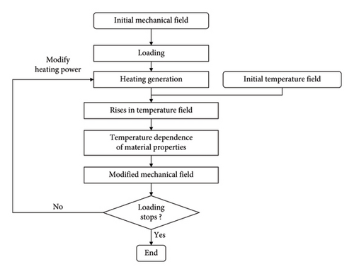
In this paper, a modeling methodology is proposed to explore the thermal-mechanical behavior of LRBs. The following techniques are included in the framework: mechanical modeling, thermal modeling, the temperature dependency of material properties, and the thermal-mechanical modeling. The modeling methodology is verified by the mechanical and thermal test data. Then, the proposed modeling methodology is employed in the detailed numerical analysis for investigating the thermal-mechanical behavior of LRBs.

2. Full-Scale Tests

2.1. Test Setup and Procedures

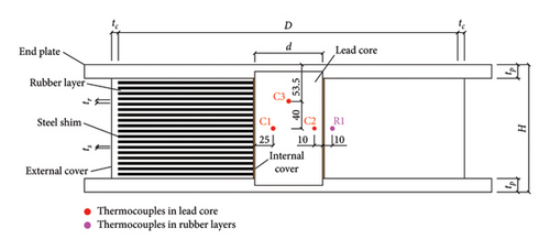
Full-scale tests were conducted to capture the coupled thermal and mechanical behavior of LRBs. The test specimen with an outer diameter of 500 mm is commonly employed in isolated buildings. The diameter of the lead core is 100 mm. The first shape factor and second shape factor are 25.5 and 5.37, respectively, which are common values in practice. The thickness of the external cover and internal cover is 10 mm and 1 mm, respectively. The internal cover is not specifically designed but formed by the vulcanization process. More detailed dimension parameters of the test specimen labeled as LRB500 are presented in Table 1.

Table 1. Dimension parameters of the test specimen labeled as LRB500.

Parameter	Symbol (unit)	Value
Bearing height	H (mm)	187
Bearing diameter	D (mm)	500
Lead core diameter	d (mm)	100
Thickness of rubber layers	t_r (mm)	4.895
Number of rubber layers	n	19
Thickness of steel shims	t_s (mm)	3
Thickness of the end plate	t_p (mm)	20
Thickness of the external cover	t_c (mm)	10
Thickness of the internal cover	t_ic (mm)	1
First shape factor	S₁ = (D − d)/(4 × t_r)	25.5
Second shape factor	S₂ = D/(n × t_r)	5.37

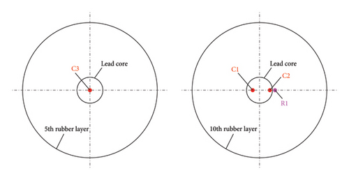
The plan and section of the LRB500 and locations of thermocouples are shown in Figure 1. The upper and lower end plates are attached to the outer rubber layers. The upper and lower parts of the lead core are embedded in the end plates. There are three thermocouples in the lead core, labeled as C1, C2, and C3. There is one thermocouple in the rubber layer, labeled as R1. The thermocouple C3 is installed at the height of the fifth rubber layer numbered from the bottom. The thermocouples C1, C2, and R1 are installed at the height of the 10th rubber layer. From the top view, C3 is located at the center of the lead core, C1 is located at the midpoint of the lead core radius, and C2 and R1 are close to the internal cover.

Details are in the caption following the image — **Figure 1 (a)**
Open in figure viewer PowerPoint

Plan and section of the LRB500 and locations of thermocouples (unit: mm). (a) Elevation. (b) Top views.

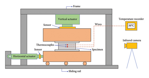
The schematic of the experimental setup is presented in Figure 2. The specimen was placed in the space between the vertical actuator and horizontal actuator. The compressive force applied on the specimen is provided by the vertical actuator. The displacement-control mode is used in the test and provided by the horizontal actuator. An initial compressive stress of 10 MPa was acted on the specimen before the horizontal loading. The real-time forces and displacements are recorded automatically by sensors attached to the two actuators. The temperature data transmission from thermocouples to the temperature recorder was implemented by wires. The temperature field on the outer surface of the specimen was monitored by the infrared camera.

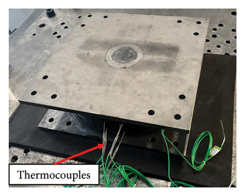
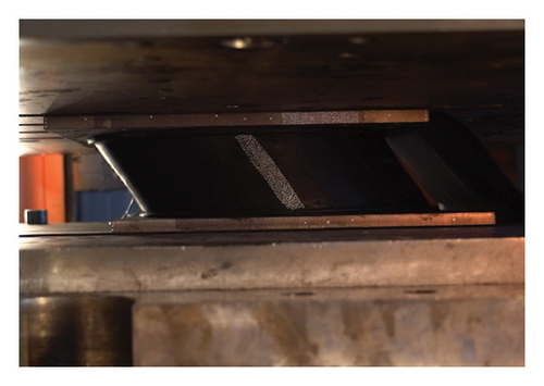
The test specimen LRB500 and its deformation under cyclic loading are shown in Figure 3. The thermocouples in the LRB500 have a diameter of only 1.5 mm, ensuring that the thermal and mechanical behaviors remain unaffected. The parameters about the test program are listed in Table 2. There are two test cases, labeled as C-1 and C-2. The case C-1 is set to investigate the mechanical behavior of the LRB500 with a very low loading speed (0.006 Hz in frequency). The case C-2 is set to investigate the thermal-mechanical behavior with a high loading speed (0.25 Hz in frequency). The shear strain and compressive stress are set to 100% and 10 MPa, respectively, for the two cases. There is an interval of over 24 h between case C-1 and case C-2.

Table 2. Test program.

Test case	Test target	Loading type	Shear strain (%)	Compressive stress (MPa)	Frequency (Hz)	Cycles
C-1	Mechanical behavior	Low speed	100	10	0.006	3
C-2	Thermal–mechanical behavior	High speed	100	10	0.25	10

2.2. Test Results and Discussion

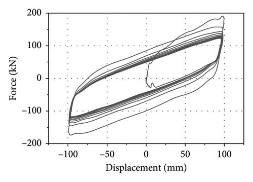
Figure 4 shows the mechanical behavior of the LRB500 in the case of C-1. As observed in Figure 4(a), there is no significant degradation in force–displacement loops as the cycle number increases. The characteristic strength (Q_d) is defined as the intercept of the force axis. The EDC is defined as the area of loops. As shown in Figures 4(b), 4(c), there is only a slight reduction in the Q_d and EDC from the first cycle to the second cycle. The mechanical behavior has exhibited stability since the second cycle. At such a low loading frequency of 0.006 Hz, most of the generated heat was transferred outward and cannot be stored in the lead core. Thus, the thermocouple recorded a very small temperature rise of no more than 5°C for the C-1 test.

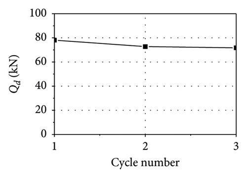
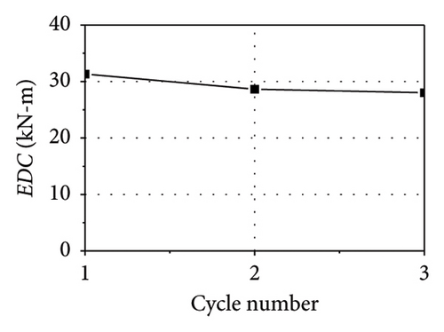
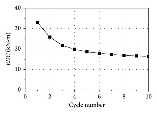
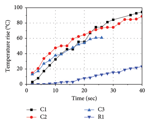
Figure 5 shows the thermal-mechanical behavior of the LRB500 in the case of C-2. As observed in Figure 5(a), there is a significant degradation in force–displacement loops as the cycle number increases. As shown in Figures 5(b), 5(c), there is a continuous reduction in the Q_d and EDC as the cycle number increases. The thermal behavior of the LRB500 is significant as observed in Figure 5(d). The temperature of measure point C1, C2, and C3 in the lead core increases rapidly with time, and the temperature rise reaches up to nearly 90°C. Note that the thermocouple in point C3 was damaged at 26 s. The temperature rise of measure point R1 in the rubber layer near the lead core reaches 22°C when the loading ends, indicating the heat has been transferred from the lead core into the rubber layers.

The infrared camera captured the infrared images of the LRB500 during the loading, as shown in Figure 6. As observed, the temperature of the outside surface of the LRB500 was 12.4°C before the loading. Note that the temperature increased to 14.1°C 12 min after the end of loading and to 16.2°C 34 min after the end of loading. The temperature of the outside surface was still rising after the loading ended, indicating that the heat was being continuously transferred from the lead core to the outside.

3. Mechanical Model

3.1. Parameters of Mechanical Models

Rubber is a typical hyperelastic material with very little compressibility compared to its shear flexibility. Hyperelastic materials are characterized by the strain energy potential (W), which quantifies the strain energy stored in the material per unit of reference volume as a function of the strain experienced at a specific point in the material. There are several models commonly employed by researchers, such as Mooney–Rivlin form [29, 31, 32], Ogden form [33, 34], and Neo–Hookean form [35]. The material models such as the Mooney–Rivlin and Neo–Hookean forms can be derived from the Ogden form, which is employed in this study because of its greater applicability than others [33]. The Ogden form is described by Equation (1) [36].

()

where

are the deviatoric principal stretches

; λ_i are the principal stretches; N is a material parameter, and μ_i are temperature-dependent material parameters. The initial shear modulus G is evaluated as Equation (2).

()

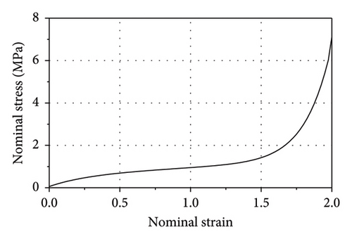
The stress-strain curve of the rubber model is plotted in Figure 7. Steel and lead are typical nearly ideal elastic-plastic material and can be described by the bilinear model. Table 3 presents the detailed parameters of mechanical models [29–33].

Table 3. Parameters of mechanical models.

Material	Mechanical model	Parameters	Value
Rubber	Ogden	μ₁	0.396 MPa
		α₁	0.12
		μ₂	0.315 MPa
		α₂	18
		μ₃	0.024 MPa
		α₃	4.84
		D₁	1.2 × 10⁻⁹ MPa⁻¹

Steel	Bilinear	Elasticity modulus	205 GPa
		Poisson ratio	0.3
		Yield stress	235 MPa

Lead	Bilinear	Elasticity modulus	17.5 GPa
		Poisson ratio	0.44
		Yield stress	15.82 MPa

3.2. Validation of the Mechanical Model

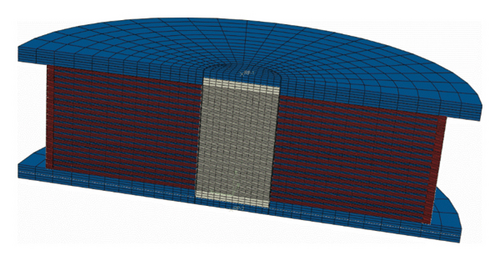
The eight-node linear hybrid element C3D8H is used to model rubber and the eight-node linear element C3D8 is used to model steel and lead. The finite element mesh is shown in Figure 8(a). Each rubber layer, steel shim, and end plate are meshed with 1920 C3D8H elements, 960 C3D8 elements, and 1800 C3D8 elements, respectively. There are 16,520 C3D8 elements in the lead core. The rubber-steel interface was modeled as a tied contact. The steel shims and rubber layers are vulcanized during manufacturing, creating a fully bonded interface with no relative motion. The rubber-lead and steel-lead interface were also modeled as a tied contact. Because the lead core is mechanically confined and experience very slight relative motion during cyclic loading. The tie contact achieves a good balance between computational cost and computational accuracy.

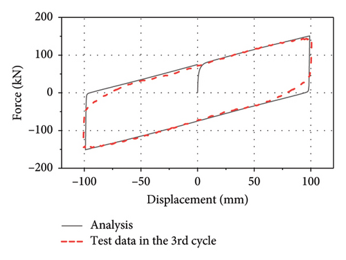
The comparison of force–displacement loops between analysis and test in the case of C-1 are shown in Figure 8(b). Dashed lines represent the test data and solid ones represent the analysis results. As observed, the implemented material models are capable of capturing the mechanical behavior with excellent accuracy.

4. Thermal Model

The thermal model is used to simulate the heating transfer process in LRBs considering the heating of the lead core. There are three primary ways to transfer heat, which are conduction, convection, and radiation. In this study, convection and radiation are not taken into account. Conduction happens because of the temperature difference within or between materials, and it is assumed to be governed by the Fourier law, described by Equation (3).

()

where k, ρ, c, T, and t are the thermal conductivity, material density, specific heat, temperature, and time, respectively; ∇ is the gradient operator; Φ^′ is the generalized heat source. The left side of Equation (3) represents the change in thermal energy, and the right side represents the heat conduction and heat source. The heat flow of LRBs is shown in Figure 9. The heat is generated in the lead core under the earthquake, and then transferred to surrounding martials by conduction.

The EDC data from case C-2 are presented in Figure 5(c). The heating power of the lead core per volume P_L can be used to represent Φ^′ and is calculated by Equation (4) [37].

()

where the constant 0.9 is the conversion coefficient from the dissipated energy to the thermal energy [38], f_z is the loading frequency in the case C-2, and V_L is the heating volume of the lead core. The thermal parameters of materials are listed in Table 4. The thermal model has the same finite element mesh as the mechanical model, as shown in Figure 8(a). All materials in the thermal model are modeled using eight-node linear heat transfer elements DC3D8. The analysis results are compared with the test data, plotted in Figure 10. As observed, the implemented thermal model is capable of capturing the thermal behavior with excellent accuracy.

Table 4. Thermal parameters.

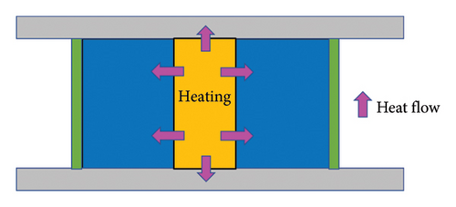
Material	Density (kg/m³)	Specific heat (J/(kg°C))	Conductivity (W/(m°C))	Element type
Steel	7800	450	50	DC3D8
Rubber	1500	1700	0.6	DC3D8
Lead	11,300	128	35	DC3D8

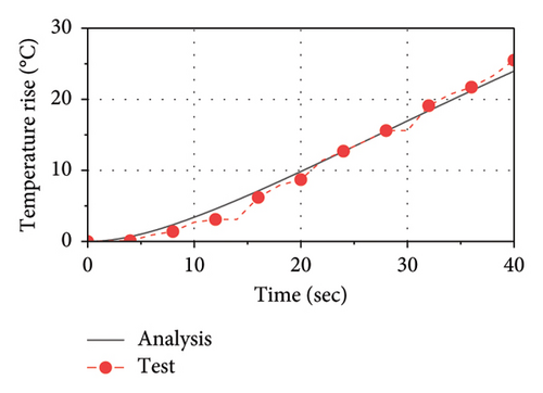
5. Temperature Dependency of Material Mechanical Properties

5.1. Steel and Rubber

The elastic modulus of steel decreases with the increasing temperature; the reduced elastic modulus E_sT can be calculated by Equations (5) and (6) [21].

()

where χ_sT is the reduction coefficient of elastic modulus, T_s is the steel temperature, and E_s is the elastic modulus at 20°C. The temperature dependency of the elastic modulus of steel is shown in Figure 11(a).

The rising temperature causes the reduction of rubber hardness. The empirical formula for the horizontal stiffness K_h(T) at temperature T (°C) can be estimated by Equation (7) [16].

()

where C(T) is the adjustment coefficient of the horizontal stiffness, and K_h(23°C) is the horizontal stiffness at 23°C. According to ISO 22762-3-2018 [6], the horizontal stiffness is derived by Equation (8).

()

where G(T) is the shear modulus, A is the cross-sectional area of the rubber bearing, and T_r is the total thickness of rubber layers. By substituting Equation (8) into Equation (7), the G(T) is given by Equation (9).

()

By substituting Equation (2) into Equation (9), the parameters μ_i(T) are obtained by Equation (10).

()

where

()

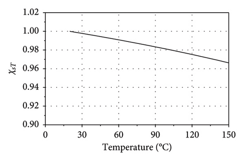
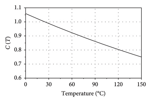
The temperature dependency of the shear modulus of rubber is shown in Figure 11(b).

5.2. Lead

In this study, the temperature dependency of mechanical properties of the lead core was investigated based on the test data and thermal analysis. The average temperature rise of the lead core ΔT_L is calculated by Equation (12).

()

where V_L is the volume of the lead core, T_i is the temperature rise at node i. V_i represents the volume of the region around the node i, assuming they share the same temperature rise (T_i). V_i is calculated based on the finite element mesh, as shown in Figure 12. The region between adjacent nodes is divided in half by the boundary lines of V_i.

The values of T_i and V_i are obtained from the analysis results of the thermal model in the case of C-2. The characteristic strength values of the LRB500 corresponding to ΔT_L are obtained from the test data in the case of C-2. The characteristic strength is primarily dependent on the yield stress of the lead core. As shown in Figure 11(c), the fitting formula regarding the temperature dependency of the characteristic strength (Q_d) is given by Equation (13).

()

6. Thermal–Mechanical Model

The thermal–mechanical model was developed by integrating the validated mechanical and thermal models, while simultaneously considering the temperature dependency of material mechanical properties. When the stress analysis depends on the temperature distribution, which in turn depends on the stress solution, a thermal–mechanical coupled analysis is required. There is a strong coupling relationship between temperature field and mechanical field in terms of LRBs. The mechanical and thermal solutions should be solved simultaneously. An exact implementation of Newton’s method involving a nonsymmetric Jacobian matrix is illustrated by Equation (14) [36].

()

where δμ and δT are the respective corrections to the incremental displacement and temperature; K_uu, K_uT, K_Tu, and K_TT are submatrices of the fully coupled Jacobian matrix; and R_u and R_T are the mechanical and thermal residual vectors, respectively.

Plastic energy dissipation of the lead core is considered as a heat source in the proposed thermal-mechanical model. The heat source in the thermal energy balance can be computed by Equation (15).

()

where η is the conversion coefficient from plastic energy dissipation to heat, σ_y and dε^p are the lead yield stress tensor and the plastic strain rate tensor respectively, “:” denotes the double dot product of tensors. Equation (15) is incorporated into the heat conduction equation (3), and a complete thermal energy balance expression in the thermal-mechanical model is given by Equation (16).

()

where the left side represents the change in thermal energy, and the right side represents heat conduction and heat source generated by plastic deformation of the lead core. The yield stress of the lead core is approximatively given by Equation (17).

()

where A_L is the cross-sectional area of the lead core. The schematic flow of the coupled analysis is shown in Figure 13. Under the loading, the heating effect of the lead core causes the rises in temperature field of LRBs. Because of the temperature dependence of material properties, the rises lead to the modified mechanical field, which in turn results in the modification in heat generation power. The coupled analysis continuously proceed until the motion of LRBs stops.

7. Numerical Results and Discussion

7.1. Validation of the Proposed Thermal–Mechanical Model

The thermal–mechanical model has the same finite element mesh as the mechanical model, as shown in Figure 8(a). The eight-node thermally coupled hybrid element with trilinear displacement and temperature C3D8HT is used to model rubber. The eight-node thermally coupled element with trilinear displacement and temperature C3D8T is used to model steel and lead.

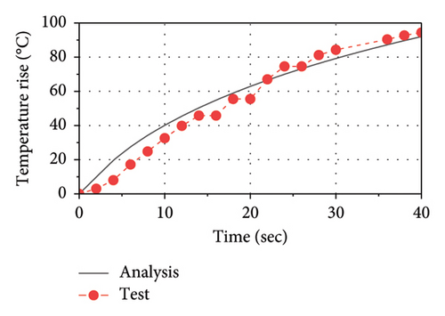
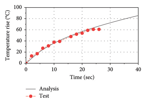
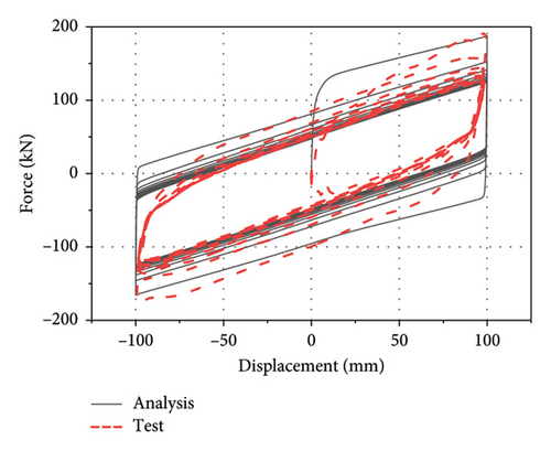
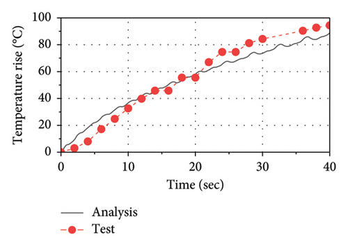
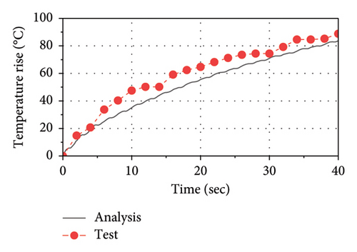
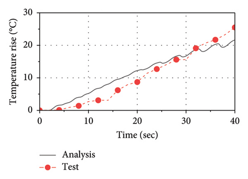
The comparison of force–displacement loops between analysis results and test data is plotted in Figure 14. As observed, the implemented thermal-mechanical model well captures the mechanical behavior of the LRB. The area of loops decreases as the number of cycles increases, indicating that the energy dissipation and the equivalent stiffness are decreasing with loading time. The comparisons of temperature rise histories between the test and the analysis at C1, C2, C3, and R1 are presented in Figure 15. As observed, the implemented thermal-mechanical model well captures the thermal behavior of the LRB500. Note that the maximum temperature rise observed inside the lead core and the rubber layer are approximately 90°C and 25°C, respectively, indicating that there is a significant heating effect in the lead core and some heat has been transferred from the lead core to rubber layers.

7.2. Influence of Temperature-Dependent Properties of Rubber and Steel

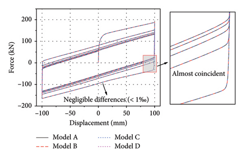
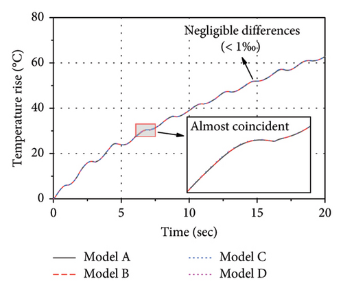
To investigate the influence of temperature dependency of rubber and steel on thermal-mechanical behavior of LRBs, three models were established, as detailed in Table 5. The temperature dependency of lead properties was considered in three models. The temperature dependency of rubber properties was considered only in the model B. The temperature dependency of steel properties was considered only in the model C. Comparisons of thermal-mechanical results among Models A (lead only), B (lead + rubber), C (lead + steel), and D (lead + rubber + steel) are shown in Figure 16. As observed, the differences between the four models are negligible (less than 1‰ deviation), no matter for the force-displacement loops or temperature rise histories. All the curves almost coincided with each other. The comparisons indicate that the influence of temperature dependency of rubber and steel on thermal-mechanical behavior of LRBs can be ignored. Thus, only the temperature dependency of lead was considered in the following analysis of this study to effectively save time in computation.

Table 5. Definition of three models.

Model type	Temperature dependency of material properties considered in the model
Model type	Lead	Rubber	Steel
Model A	Yes
Model B	Yes	Yes
Model C	Yes		Yes
Model D	Yes	Yes	Yes

7.3. Plastic Strain and Temperature Field of the Lead Core

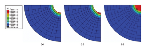
Figure 17 shows the equivalent plastic strain (PEEQ) of the lead core as the lateral displacement reaches the maximum value. The overall and close-up views are shown in Figures 17(a), 17(b), respectively. The plastic strain distribution inside the lead core is far from uniform; the PEEQ in the regions at the same height as rubber layers is significantly larger than in the regions at the same height as steel shims. This is because the stiffness of rubber is much lower than that of steel. Steel shims impose a strong constraint on the adjacent lead core region, thereby inhibiting the occurrence of plastic strain in those regions.

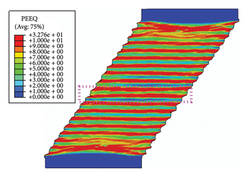
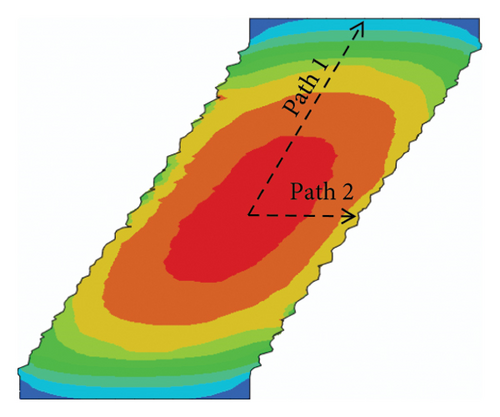
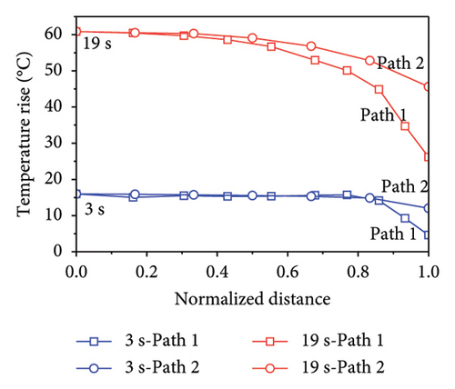
Figure 18 shows the temperature rise field of the lead core as the lateral displacement reaches the maximum value. The temperature rise fields at first and fifth cycles are shown in Figures 18(a), 18(b), respectively. The temperature distribution of the first cycle inside the lead core is uniform. However, the lead core gradually exhibits a gradient-distributed temperature rise field from the inside to the outside because of the cumulative effect of heat. The one-dimensional temperature rise fields along specified path 1 and path 2 are plotted in Figure 18(c). As observed, the temperature rises along path 1 and path 2 are uniform when the loading time t = 3 s. As time t reaches up to 19s, the temperature rises along the path 1 and path 2 decrease significantly with the distance. The temperature rises at the end of path 1 and path 2 are reduced by 60% and 25%, respectively, compared to the temperature rise at the start point of paths.

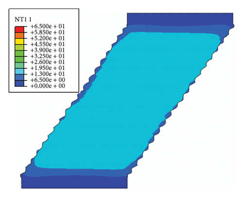
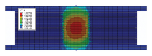
The temperature rise field of the LRB500 at the 10th cycle is shown in Figure 19. As observed, the majority of generated heat is stored in the lead core when the loading ends. Some of the heat is transferred into the rubber layers, steel shims, and end plates, as shown in Figure 20. The heat reaches the upper and lower boundaries of the LRB500, while no heat reaches the peripheral boundary of the LRB500. The numerical model focused on coupled thermal-mechanical behavior during seismic loading (lasting 40 s in this analysis), not the post-earthquake heat conduction. Consequently, the simulation did not capture the slow conduction of residual heat to the outer surface, which was observed experimentally in Figure 6.

7.4. Parametric Analysis

Figure 21 shows the influence of the lead core diameter (d) on thermal-mechanical behaviors of the LRB500. As observed, as the d varies from 100 mm to 120 mm, although the rate of energy accumulation is significantly increased, there is only a very slight increase in the temperature rise rate of the lead core. Thus, the variation in the lead core diameter primarily influences the mechanical behavior rather than the thermal behavior of the LRB500.

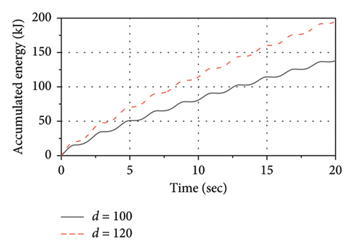
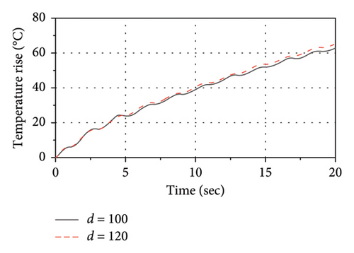
Figure 22 shows the influence of the compressive stress (σ) on thermal-mechanical behaviors of the LRB500. As observed, as the σ varies from 5 MPa to 10 MPa, the increase in both the rate of energy accumulation and the temperature rise rate of the lead core is very slight. Thus, the variation in the compressive stress has no significant influence on either the mechanical behavior or thermal behavior of the LRB500.

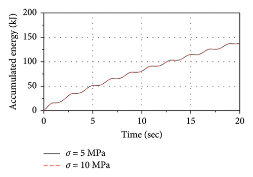
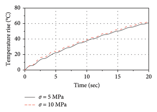
Figure 23 shows the influence of the loading frequency (f) on thermal-mechanical behaviors of the LRB500. As observed, as the f varies from 0.25 Hz to 0.5 Hz, the increase in both the rate of energy accumulation and the temperature rise rate of the lead core is significant. Thus, the variation in the loading frequency has a significant influence on both the mechanical behavior and thermal behavior of the LRB500.

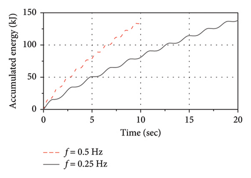
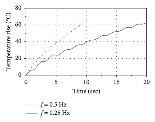
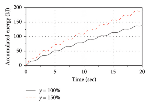
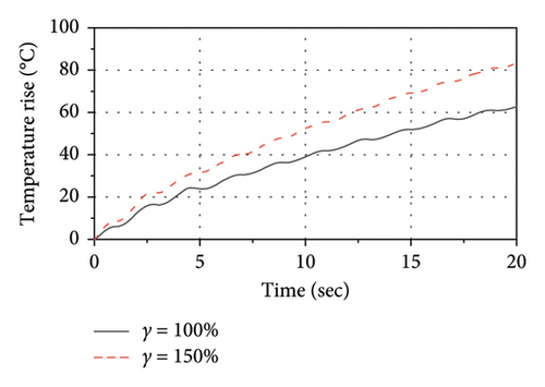
Figure 24 shows the influence of the shear strain (γ) on thermal-mechanical behaviors of the LRB500. As observed, as the γ varies from 100% to 150%, the increase in both the rate of energy accumulation and the temperature rise rate of the lead core is significant. Thus, the variation in the shear strain has a significant influence on both the mechanical behavior and thermal behavior of the LRB500.

7.5. Thermal–Mechanical Behavior of LRBs Subjected to a Nonharmonic Motion History

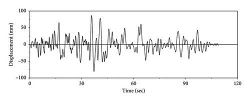
A case study was performed on the LRB500 subjected to a nonharmonic horizontal motion history with a constant compressive stress of 10 MPa, to assess the differences between thermal-mechanical and mechanical models of LRBs. The history of the imposed motion is presented in Figure 25. As observed, the peak displacement reached 85 mm, which is corresponding to a shear strain (equal to the lateral displacement divided by the total thickness of rubber) of about 100%. This level of shear strain is considered an expected and reasonable behavior for LRBs under a design basis earthquake [7].

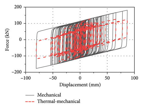
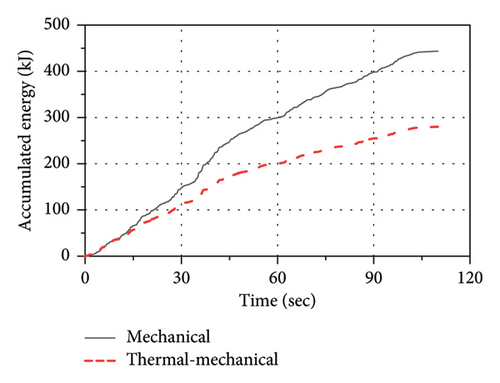
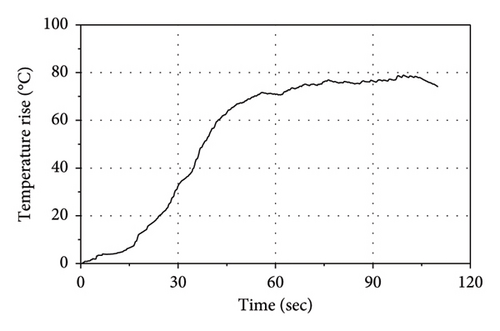
The nonharmonic motion displacement history was imposed to both the thermal–mechanical and mechanical models. The comparisons of force–displacement loops and the accumulated energy between the thermal–mechanical and mechanical models are shown in Figure 26. As observed in Figure 26(a), the force–displacement loops of the thermal–mechanical model are significantly different from those of the mechanical model. In the thermal–mechanical model, the intercept of the force axis of loops (characteristic strength of LRBs) continuously decreases with the cycles, where it remained constant in the mechanical model. As observed in Figure 26(b), the thermal–mechanical model has a significantly lower rate in the accumulated energy than the mechanical model. The final energy dissipation of the thermal–mechanical model amounts to only 63% of that exhibited by the mechanical model. The conventional mechanical model overestimates the energy dissipation of the LRB500, and thus could underestimate seismic responses under the earthquake. Figure 27 shows the temperature rise history of lead core center in the thermal–mechanical model. The temperature exhibits an initial rapid increase, followed by a gradual stabilization in the later stages. The final temperature rise at lead core center reaches nearly 80°C.

8. Conclusions

In this study, the thermal-mechanical behavior of LRBs is investigated by full-scale testing and numerical analysis. A modeling methodology is proposed to explore the thermal-mechanical behavior of LRBs. The following conclusions can be drawn:

1.
The full-scale testing results indicate a significant mechanical degradation and a substantial rise of nearly 90°C in the temperature field of LRBs under the high-speed loading. Moreover, the temperature rises in the outside surface of the LRB are observed from the infrared images.
2.
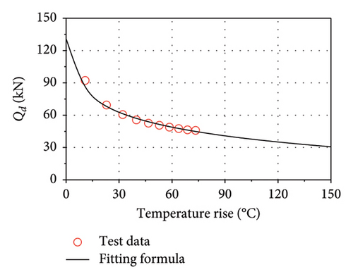
The temperature dependency of mechanical properties of the lead core is obtained based on the test data and thermal analysis. The thermal-mechanical model using the proposed modeling methodology can accurately predict the thermal and mechanical test data.
3.
The numerical analysis shows that there is a gradient-distributed temperature rise field from the center of the lead core outwards. The thermal–mechanical behavior of LRBs is sensitive to the shear strain and loading frequency.
4.
A case study conducted in this paper shows that the thermal–mechanical coupling effect of LRBs under a nonharmonic motion history is significant. The conventional mechanical model may overestimate the seismic performance of LRBs, and thus could underestimate seismic responses under the earthquake.

Conflicts of Interest

The authors declare no conflicts of interest.

Author Contributions

Bin Xue: conceptualization, methodology, formal analysis, investigation, software, writing – original draft, and writing and review–editing. Wensheng Lu was in charge of conceptualization, resources, writing and review–editing, and supervision. Xiangxiang Ren: conceptualization, resources, writing and review–editing, and supervision. Wenlu Wen: investigation, writing – original draft, and writing and review–editing.

Funding

This work was supported by the National Natural Science Foundation of China (52308527) and Natural Science Foundation of Chongqing, China (CSTB2022NSCQ-MSX0476).

Acknowledgments

This work was supported by the National Natural Science Foundation of China (52308527) and Natural Science Foundation of Chongqing, China (CSTB2022NSCQ-MSX0476).

Open Research

Data Availability Statement

The data that support the findings of this study are available from the corresponding author upon reasonable request.

References

1 Sato E., Furukawa S., Kakehi A., and Nakashima M., Full-Scale Shaking Table Test for Examination of Safety and Functionality of Base-Isolated Medical Facilities, Earthquake Engineering & Structural Dynamics. (2011) 40, no. 13, 1435–1453, https://doi.org/10.1002/eqe.1097, 2-s2.0-80052952917.
10.1002/eqe.1097
Web of Science® Google Scholar
2 De Luca A. and Guidi L. G., State of Art in the Worldwide Evolution of Base Isolation Design, Soil Dynamics and Earthquake Engineering. (2019) 125, https://doi.org/10.1016/j.soildyn.2019.105722, 2-s2.0-85068553314.
10.1016/j.soildyn.2019.105722
Web of Science® Google Scholar
3 Junwu D., Wen B., Baofeng Z., and Rongheng L., Urgent Problems Need to Be Solved in the Development of Seismic Base Isolation for Buildings From the Luding Ms6.8 Earthquake, Earthquake Engineering and Engineering Dynamics. (2022) 42, no. 6, 1–11, https://doi.org/10.13197/j.eeed.2022.0601.
10.13197/j.eeed.2022.0601
Google Scholar
4 Bhatta S., Kang X., and Dang J., Machine Learning Prediction Models for Ground Motion Parameters and Seismic Damage Assessment of Buildings at a Regional Scale, Resilient Cities and Structures. (2024) 3, no. 1, 84–102, https://doi.org/10.1016/j.rcns.2024.03.001.
10.1016/j.rcns.2024.03.001
Google Scholar
5 Zhang R. J. and Li A. Q., Probability Distribution Characteristics and Statistical Parameters of the Horizontal Stiffness of Rubber Isolation Bearings, Journal of Earthquake Engineering. (2022) 26, no. 5, 2437–2449, https://doi.org/10.1080/13632469.2020.1762806.
10.1080/13632469.2020.1762806
Web of Science® Google Scholar
6 ISO, Elastomeric Seismic-Protection Isolators (IOS 22762-3), 2018, ISO.
Google Scholar
7 China Planning Press, Standard for Seismic Isolation Design of Building (GB/T 51408-2021), 2021, China Planning Press.
Google Scholar
8 American Society of Civil Engineers, Minimum Design Loads and Associated Criteria for Buildings and Other Structures, 2016, American Society of Civil Engineers.
Google Scholar
9 He W. F., Luo H. J., Chang W. H., Xu H., Liu W. G., and Zhang Q., Experiment Investigation and in Situ Test of Hybrid Vibration Bearing System Applied to Overtrack Historical Buildings, Structural Control and Health Monitoring. (2022) 29, no. 4, https://doi.org/10.1002/stc.2921.
10.1002/stc.2921
PubMed Web of Science® Google Scholar
10 Zhang R. F., Wu M. J., Lu W. S., Li X., and Lu X. L., Seismic Retrofitting of a Historic Building by Using an Isolation System With a Weak Restoring Force, Soil Dynamics and Earthquake Engineering. (2021) 148, https://doi.org/10.1016/j.soildyn.2021.106836.
10.1016/j.soildyn.2021.106836
Web of Science® Google Scholar
11 Vasiliadis L. K., Seismic Evaluation and Retrofitting of Reinforced Concrete Buildings With Base Isolation Systems, Earthquakes and Structures. (2016) 10, no. 2, 293–311, https://doi.org/10.12989/eas.2016.10.2.293, 2-s2.0-84962835248.
10.12989/eas.2016.10.2.293
Web of Science® Google Scholar
12 Wang L., Nagarajaiah S., Shi W., and Zhou Y., Seismic Performance Improvement of Base-Isolated Structures Using a Semi-Active Tuned Mass Damper, Engineering Structures. (2022) 271, https://doi.org/10.1016/j.engstruct.2022.114963.
10.1016/j.engstruct.2022.114963
Web of Science® Google Scholar
13 Wang B., Karavasilis T. L., Chen P., and Dai K., Seismic Modeling and Performance Evaluation of Seismically Isolated Building Considering Large Strain Effects Under Near-Fault Earthquakes, Journal of Building Engineering. (2024) 90, https://doi.org/10.1016/j.jobe.2024.109339.
10.1016/j.jobe.2024.109339
Web of Science® Google Scholar
14 Wang B., Chen P., Zhu S. Y., and Dai K. S., Seismic Performance of Buildings With Novel Self-Centering Base Isolation System for Earthquake Resilience, Earthquake Engineering & Structural Dynamics. (2023) 52, no. 5, 1360–1380, https://doi.org/10.1002/eqe.3820.
10.1002/eqe.3820
Web of Science® Google Scholar
15 Xu G., Guo T., Li A. Q., Zhang R. J., Zhu R. Z., and Liu F. Q., Influence of Ambient Temperature on Seismic Performance of Elastomeric Isolation Structural System, Structures. (2023) 55, 1763–1773, https://doi.org/10.1016/j.istruc.2023.06.130.
10.1016/j.istruc.2023.06.130
Web of Science® Google Scholar
16 Pang H., Jiang T., Dai J., Yang Y., and Bai W., Experimental Study of the Mechanical Properties of Full-Scale Rubber Bearings at 23°C, 0°C, and −20°C, Polymers. (2024) 16, no. 7, https://doi.org/10.3390/polym16070903.
10.3390/polym16070903
Google Scholar
17 Zhu L. H., Meng L. F., Dong Y. R., Su H., and Jia W., Study on the Performance Degradation of LRB Under the Combination of Low Temperature Cycles and Superstructure Weight, Journal of Earthquake Engineering. (2024) 28, no. 10, 2763–2780, https://doi.org/10.1080/13632469.2024.2305765.
10.1080/13632469.2024.2305765
Web of Science® Google Scholar
18 Yasar C., Karuk V., Cavdar E., and Ozdemir G., Modifications in Both Lead and Rubber Properties of Lrbs at Low Temperatures Considering the Size Effect, Engineering Structures. (2024) 307, https://doi.org/10.1016/j.engstruct.2024.117902.
10.1016/j.engstruct.2024.117902
Web of Science® Google Scholar
19 Chu H., Xu K., Huang W., and Cai L., Heat-Generating of Rubber and Its Influence on Mechanical Properties, Journal of Beijing University of Technology. (2017) 43, no. 11, 1635–1640.
Google Scholar
20 Shi W., Zhang K., Tan Z., and Chen J., Influence of Variable Temperature Environment on Mechanical Properties of Rubber, Polymer Materials Science and Engineering. (2021) 37, no. 11, 110–116.
CAS Google Scholar
21 China Planning Press, Code for Fire Safety of Steel Structures in Buildings (GB51249-2017), 2018, China Planning Press.
Google Scholar
22 Kalpakidis I. V. and Constantinou M. C., Effects of Heating on the Behavior of Lead-Rubber Bearings. I: Theory, Journal of Structural Engineering. (2009) 135, no. 12, 1440–1449, https://doi.org/10.1061/(ASCE)ST.1943-541X.0000072, 2-s2.0-70450197211.
10.1061/(ASCE)ST.1943-541X.0000072
Web of Science® Google Scholar
23 Guruswamy S., Engineering Properties and Applications of Lead Alloys, 1999, CRC Press.
10.1201/9781482276909
Google Scholar
24 Pourmasoud M., Hajirasouliha I., Park A., and Lim J., A New Approach to Estimate the Lead Core Characteristic Strength of Lead Rubber Bearings, Engineering Structures. (2022) 270, https://doi.org/10.1016/j.engstruct.2022.114817.
10.1016/j.engstruct.2022.114817
Web of Science® Google Scholar
25 Ozdemir G., Formulations of Equivalent Linearization of Lead-Rubber Bearings for Incorporating the Effect of Lead Core Heating, Earthquake Spectra. (2015) 31, no. 1, 317–337, https://doi.org/10.1193/041913eqs107m, 2-s2.0-84922749017.
10.1193/041913eqs107m
Web of Science® Google Scholar
26 Wake T., Kikuchi M., and Ishii K., Strength Degradation in Lead-Rubber Bearings During a Long-Duration Earthquake, Proceedings of the NZSEE Conference, 2017, New Zealand.
Google Scholar
27 Kalpakidis I. V., Effects of Heating and Load History on the Behavior of Lead-Rubber Bearings, 2008, State University of New York at Buffalo.
Google Scholar
28 Liu Y. H., Zhong W. J., Mercan O., Tan P., and Zhou F. L., A New Nonlinear Model to Describe the Degradation Law of the Mechanical Properties of Lead-Rubber Bearings Under High-Speed Horizontal Loading, Structural Control and Health Monitoring. (2021) 28, no. 12, https://doi.org/10.1002/stc.2836.
10.1002/stc.2836
PubMed Web of Science® Google Scholar
29 Ren X. X., Lu W. S., Zhu Y. H., He Y., and Li T. G., Compressive Behavior of Low Shape Factor Lead-Rubber Bearings: Full-Scale Testing and Numerical Modeling, Engineering Structures. (2020) 209, https://doi.org/10.1016/j.engstruct.2019.110030.
10.1016/j.engstruct.2019.110030
Web of Science® Google Scholar
30 Zhang Z. D., Zhou Y., and Vassiliou M. F., Experimental, Numerical, and Theoretical Studies on Vertical Stiffness Reduction of Lead Thick Rubber Bearings, Construction and Building Materials. (2023) 384, https://doi.org/10.1016/j.conbuildmat.2023.131421.
10.1016/j.conbuildmat.2023.131421
Web of Science® Google Scholar
31 Xue B., Lu W., and Ren X., Refined Lead Boundary Simulation for Compressive Behavior of Low–Shape Factor Lead-Rubber Bearings, Journal of Structural Engineering. (2023) 149, no. 6, https://doi.org/10.1061/jsendh.steng-11994.
10.1061/jsendh.steng-11994
Web of Science® Google Scholar
32 Ahmadipour M. and Alam M. S., Sensitivity Analysis on Mechanical Characteristics of Lead-Core Steel-Reinforced Elastomeric Bearings Under Cyclic Loading, Engineering Structures. (2017) 140, 39–50, https://doi.org/10.1016/j.engstruct.2017.02.014, 2-s2.0-85014616975.
10.1016/j.engstruct.2017.02.014
Web of Science® Google Scholar
33 Ohsaki M., Miyamura T., Kohiyama M., Yamashita T., Yamamoto M., and Nakamura N., Finite-Element Analysis of Laminated Rubber Bearing of Building Frame Under Seismic Excitation, Earthquake Engineering & Structural Dynamics. (2015) 44, no. 11, 1881–1898, https://doi.org/10.1002/eqe.2570, 2-s2.0-84938968324.
10.1002/eqe.2570
Web of Science® Google Scholar
34 Kalfas K. N., Mitoulis S. A., and Katakalos K., Numerical Study on the Response of Steel-Laminated Elastomeric Bearings Subjected to Variable Axial Loads and Development of Local Tensile Stresses, Engineering Structures. (2017) 134, 346–357, https://doi.org/10.1016/j.engstruct.2016.12.015, 2-s2.0-85008429059.
10.1016/j.engstruct.2016.12.015
Web of Science® Google Scholar
35 Toopchi-Nezhad H., Tait M. J., and Drysdale R. G., Bonded Versus Unbonded Strip Fiber Reinforced Elastomeric Isolators: Finite Element Analysis, Composite Structures. (2011) 93, no. 2, 850–859, https://doi.org/10.1016/j.compstruct.2010.07.009, 2-s2.0-79951513689.
10.1016/j.compstruct.2010.07.009
Web of Science® Google Scholar
36 Systèmes D., Abaqus Analysis User’s Guide 6.14, Dassault Systèmes.
Google Scholar
37 Xue B., Lu W., Ren X., and Wen W., A Hysteretic Model of Lead-Rubber Bearings Considering Coupled Thermal and Mechanical Behavior, Journal of Building Engineering. (2025) 103, https://doi.org/10.1016/j.jobe.2025.112118.
10.1016/j.jobe.2025.112118
Web of Science® Google Scholar
38 Majidi O., Barlat F., and Lee M.-G., Effect of Slide Motion on Springback in 2-D Draw Bending for AHSS, International Journal of Material Forming. (2016) 9, no. 3, 313–326, https://doi.org/10.1007/s12289-014-1214-7, 2-s2.0-84922346377.
10.1007/s12289-014-1214-7
Web of Science® Google Scholar

All articles

Coupled Thermal and Mechanical Behavior of Lead–Rubber Bearings: Full-Scale Testing and Numerical Modeling Methodology

Abstract

1. Introduction

2. Full-Scale Tests

2.1. Test Setup and Procedures

2.2. Test Results and Discussion

3. Mechanical Model

3.1. Parameters of Mechanical Models

3.2. Validation of the Mechanical Model

4. Thermal Model

5. Temperature Dependency of Material Mechanical Properties

5.1. Steel and Rubber

5.2. Lead

6. Thermal–Mechanical Model

7. Numerical Results and Discussion

7.1. Validation of the Proposed Thermal–Mechanical Model

7.2. Influence of Temperature-Dependent Properties of Rubber and Steel

7.3. Plastic Strain and Temperature Field of the Lead Core

7.4. Parametric Analysis

7.5. Thermal–Mechanical Behavior of LRBs Subjected to a Nonharmonic Motion History

8. Conclusions

Conflicts of Interest

Author Contributions

Funding

Acknowledgments

Open Research

Data Availability Statement

References

Figures

References

Information

About Wiley Online Library

Help & Support

Opportunities

Connect with Wiley

Coupled Thermal and Mechanical Behavior of Lead–Rubber Bearings: Full-Scale Testing and Numerical Modeling Methodology

Abstract

1. Introduction

2. Full-Scale Tests

2.1. Test Setup and Procedures

2.2. Test Results and Discussion

3. Mechanical Model

3.1. Parameters of Mechanical Models

3.2. Validation of the Mechanical Model

4. Thermal Model

5. Temperature Dependency of Material Mechanical Properties

5.1. Steel and Rubber

5.2. Lead

6. Thermal–Mechanical Model

7. Numerical Results and Discussion

7.1. Validation of the Proposed Thermal–Mechanical Model

7.2. Influence of Temperature-Dependent Properties of Rubber and Steel

7.3. Plastic Strain and Temperature Field of the Lead Core

7.4. Parametric Analysis

7.5. Thermal–Mechanical Behavior of LRBs Subjected to a Nonharmonic Motion History

8. Conclusions

Conflicts of Interest

Author Contributions

Funding

Acknowledgments

Open Research

Data Availability Statement

References

Figures

References

Related

Information