Digital Twin-Empowered Analysis of Structural Temperature Field of a Long-Span Suspension Bridge
Abstract
Structural temperature field significantly affects structural responses, such as displacements and stresses, of a long-span suspension bridge. An accurate and effective analysis of structural temperature field is therefore important. This study proposes a digital twin-empowered analysis of structural temperature field of a long-span suspension bridge. The real bridge and its surrounding environment are regarded as a physical entity. The information, such as ambient temperature and structural temperature, collected by the structural health monitoring system at the locations of sensors is taken as the data collected from the physical entity. A 3D finite element model of the bridge is then constructed as a virtual entity for heat transfer analysis with solar radiation, wind speed, and other environmental conditions included. The data collected from the physical entity are then mapped to the virtual entity through a particle swarm optimization algorithm to update uncertain parameters in the thermal boundary and convert the virtual entity to a digital twin. The established digital twin is finally used to find and predict the structural temperature field of the entire bridge. The results demonstrate that the digital twin-empowered heat transfer analysis is feasible and able to provide more accurate prediction of the structural temperature field of the entire bridge.
1. Introduction
As a kind of special structure that spans over rivers, valleys, or seas on the earth, a long-span suspension bridge often exists in a unique natural environment and constantly exchanges heat with the environment [1, 2]. As the solar radiation and air temperature in the environment surrounding the bridge undergo daily and seasonal changes, the nonuniform structural temperature field of the entire bridge also changes accordingly. The nonuniform structural temperature field inevitably causes the expansion and contraction of the bridge components, and excessive structural constraints to such expansion and contraction will then cause excessive temperature stresses in the bridge components [3–7]. Some studies have shown that the effects of temperature on structural stability and durability are sometimes greater than those made by other operational loads [8, 9]. Therefore, an in-depth study of the structural temperature field is of great significance for the functionality and safety of a long-span suspension bridge.
Owing to the complicated structural system and complex heat flow boundary of a long-span suspension bridge, it becomes unrealistic to obtain the analytical solution of the structural temperature field of the bridge only through theoretical analysis. There are two common methods currently available for determining the structural temperature distribution of the bridge. One refers to numerical simulation and analysis [10–13]. One-dimensional (1D) models of bridge components were initially established to consider heat transfer in a single direction of a structural component. Two-dimensional (2D) models were then established to consider the temperature gradient in the transverse and vertical directions of a structural component. Later, three-dimensional (3D) models were established to consider the 3D heat transfer within a structural component [14]. However, these simplified analyses cannot consider the heat transfer behavior between bridge components, and they are difficult to simulate the structural temperature distribution of the entire bridge. Subsequently, some scholars established 3D finite element (FE) models of the entire bridge for heat transfer analysis to obtain an intuitive temperature field distribution of the entire bridge [11, 15, 16].
The thermal boundary conditions of a 3D FE model of the entire bridge are quite complex and affected by various factors such as ambient temperature, solar radiation, and wind speed. Empirical parameters and formulas are therefore necessitated to determine thermal boundary conditions in heat transfer analysis. Previous studies have indicated that variations in solar radiation across different structural surfaces are the primary cause of structural temperature differences [11, 13]. Because the variations in solar radiation are influenced by many factors such as solar trajectory, incident angle, atmospheric clarity, and shading presence or absence, the effects of solar radiation on structural temperature differences are quite complex. Consequently, in previous studies, these factors were typically incorporated into FE models using some empirical geometric relationships [17]. Some scholars considered shading relationships using shadow recognition technology. Xia et al. [18] used the radiation matrix provided by ANSYS for recognition, but the scale of structures was small. When this algorithm is used to recognize complex and large-scale FE models, the computational efficiency becomes a bottleneck. Manconi and Moonen [16] performed shadow recognition through ladybug tools in Rhino and then introduced the recognition results into the FE model for calculation through the ABAQUS subroutine. This method can conduct shadow analysis with the aid of mature sunlight analysis programs, but it involves multiple software platforms, and the import is cumbersome and occupies a large amount of computer memory. Wang et al. [19] used ray tracing technology to perform shadow recognition on a complex truss arch rib segment and conducted thermal analysis of the entire arch ring. The computation speed has been effectively improved by using this method, but it has not been applied to the entire long-span suspension bridge.
Nevertheless, there is currently a lack of unified formulas to guide the determination of other parameters, leading to a reliance on individual experience for estimating these parameters. This inevitably introduces a high degree of uncertainty, thereby affecting the accuracy and reliability of the heat transfer analysis results. Furthermore, due to the inherent complexity and uncertainty of the physical world, these parameters are not static but vary with time, seasons, and climatic conditions. These parameters are highly correlated with the processes of heat dissipation and accumulation, and their inaccurate approximations may lead to significant errors in the calculated structural temperature distributions.
To this end, another way is to install a structural health monitoring (SHM) system in a long-span suspension bridge with temperature sensors to obtain the structural temperature of the bridge [18, 20, 21]. The structural temperature measured by temperature sensors is the real temperature of the bridge, but it is limited by the number of sensors. The structural temperature data obtained by the SHM system are therefore always limited to a few points of the bridge and cannot provide a complete structural temperature field for the entire bridge. Since the temperature effect on the bridge is often global behavior, even if the real temperature at a few points is obtained, it is still difficult to be used for the subsequent temperature effect analysis.
In this regard, the concept of digital twins will be used in this study to inherently integrate the numerical simulation with the temperature measured at a few points of the bridge for making a better estimation of the parameters in thermal boundary conditions and updating the 3D FE model regularly so that an accurate and varying structural temperature field can be provided for the entire bridge. The digital twin technology, as a cutting-edge technology, has been applied to bridge engineering. For example, Lin et al. [22] created a digital twin for collapse fragility assessment of a long-span cable-stayed bridge under strong earthquakes. Zhang et al. [23] developed a digital twin for the vortex-induced vibration of an in-service long-span suspension bridge. Liang et al. [24] developed a digital twin for the dynamics of a coupled train-track-bridge system. Nevertheless, the domain of structural temperature fields of long-span bridges within the context of digital twins remains relatively unexplored.
This study is therefore dedicated to a digital twin-empowered analysis of structural temperature field of a long-span suspension bridge. The remaining parts of this paper are as follows. Section 2 introduces the basic steps for a digital twin-empowered analysis. Section 3 presents a real large-span suspension bridge with a SHM system as a physical entity and collects the relevant measurement data from the physical entity. Section 4 establishes a 3D FE model of the bridge as a virtual entity for simulating its structural temperature field with a refined heat transfer analysis and an automated execution of thermal boundary conditions from the measurement data. Section 5 integrates the relevant measurement data collected from the physical entity with the virtual entity through a particle swarm optimization (PSO) algorithm to update uncertain parameters in the thermal boundary and convert the virtual entity to a digital twin. Section 6 verifies the digital twin and predicts the spatial distribution of the structural temperature field of the entire long-span suspension bridge. Section 7 summarizes the research findings and conclusions.
2. Basic Steps for Digital Twin-Empowered Analysis
- 1.
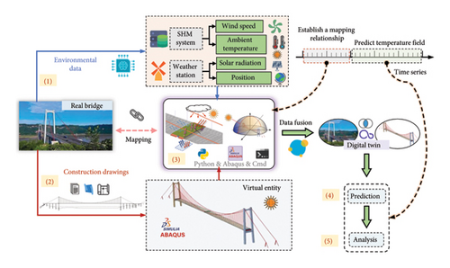
Select a real long-span suspension bridge equipped with a SHM system as a physical entity and collect the relevant information, such as ambient temperature and structural temperature, from the physical entity.
- 2.
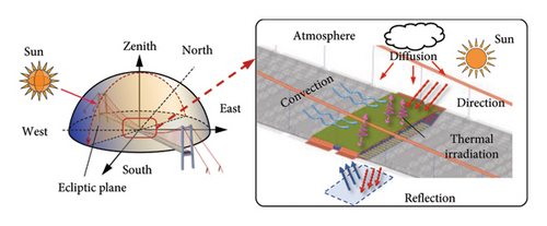
Develop a 3D FE model of the bridge and perform the heat transfer analysis for structural temperature field of the bridge. The environmental data obtained from the real bridge will be transformed into the thermal boundary conditions for the 3D FE model through a Python–Fortran secondary development program. This secondary development program will establish a virtual Sun based on geographical information and solar radiation data and perform a real-time shadow identification for the bridge. According to the identification results, it will automatically calculate the solar radiation heat flux on the bridge surface and apply convective and radiative heat flux based on the measured wind speed and direction and ambient temperature. The 3D FE model with the heat transfer analysis is regarded as a virtual entity in this study.
- 3.
Map the measured structural temperatures at several locations of the bridge to the virtual entity to form a digital twin. That is, use the measured structural temperature to update the uncertain parameters in the thermal boundary condition during the heat transfer analysis using the PSO algorithm. During the updating process, the measured structural temperature data from the sensors are used to continuously correct the calculated temperature values of the virtual entity, leading the calculated values to converge to the measured values, and thereby gradually establishing a mapping relationship between the physical entity and the virtual entity and finally forming a digital twin. This process is implemented automatically by the combination of several commercial software.
- 4.
Use the digital twin established in Step 3 to simulate the structural temperature field of the entire bridge for the next few days and compare the results with the measured structural temperature on the same days to demonstrate the prediction capacity of the digital twin.
- 5.
Use the constructed digital twin to provide the time-varying structural temperature field of the entire long-span suspension bridge.
3. A Long-Span Suspension Bridge and Physical Entity
3.1. Long-Span Suspension Bridge
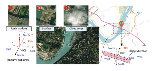
This study takes a long-span suspension bridge in southwestern China as a physical entity for a digital twin-empowered analysis of structural temperature field. The bridge, located at 28.78°N and 104.94°E, spans the Yangtze River in the east–west direction, as illustrated in Figure 2, in the world coordinate system (WCS) with the z-axis in the south, the x-axis in the east, and the y-axis upward. The bridge coordinate system (BCS), which takes the bridge longitudinal axis as the x-axis, is derived by rotating WCS counterclockwise by 160° around the y-axis of WCS. The bridge site is located in a subtropical humid climate zone, characterized by dry springs and hot summers with abundant rainfall primarily between May and September. The surrounding environment of the bridge is predominantly aquatic, with a sandbar in the river center, wetland topography on the west bank, and densely vegetated hills on the east bank, presenting a diverse range of surface conditions. The thermal environment of the bridge is influenced by the diurnal variation of solar trajectory and the dynamic impact of atmospheric clouds on solar radiation, resulting in time-varying sunlit shadows. These factors, along with topography and water distribution, contribute to the complexity of the thermal boundary conditions of the bridge, posing challenges to the heat transfer studies.
The configuration of the bridge is detailed in Figure 3, featuring a total length of 1260 m and a main span L of 820 m with a rise span ratio of 1:10. The towers are H-shaped reinforced concrete structures of 128 m in height with a top elevation of 400.61 m. The stiffened deck of the bridge is of steel box girder construction with a deck width of 29.78 m, designed for a four-lane dual carriageway and surfaced with asphalt concrete, and with a design elevation at the midspan of 314.61 m. The main cables of the bridge are composed of parallel wire strands (PPWS), made up of high-strength galvanized steel wires, and are externally coated with a protective layer. Suspenders, which connect the main cables to the main girder, are made of the same material as the main cables and are externally wrapped with a PE layer.

3.2. SHM System
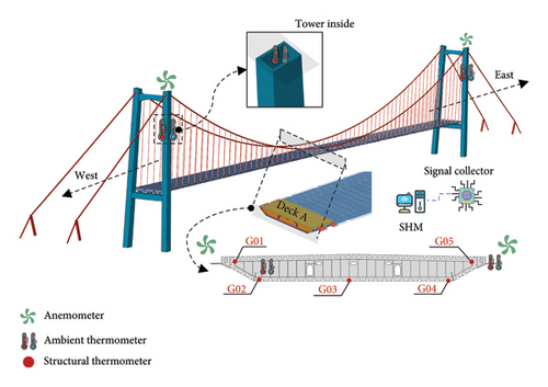
A SHM system was designed and installed on the bridge. The relevant sensors and their locations in the SHM system of the bridge are shown in Figure 4. Ambient temperature sensors were installed inside and outside the girder at the midspan of the bridge and inside the north and south towers to measure the ambient temperature inside the box chambers. The sampling frequency of the ambient temperature sensors is 1/600 Hz. Anemometers were installed at the midspan of the bridge deck and the top of the bridge towers to measure wind speed and direction at different positions of the bridge. Among them, two 3D ultrasonic anemometers were installed at the midspan of the bridge deck on the north side and south side, respectively, with a sampling frequency of 20 Hz, while a mechanical anemometer was installed at the top of each tower with a sampling frequency of 1/600 Hz. Five structural temperature sensors were installed inside the box girder in Section A at the midspan of the bridge deck to measure the structural temperatures at different positions. Specifically, sensors G01 and G05 are located on a diaphragm plate adjacent to the top plate, while sensors G02, G03, and G04 are located directly on the bottom plate. The sensors were installed with a sampling frequency of 1/600 Hz.
3.3. Measurement Information Collected From Physical Entity
The environmental monitoring data for five days from 00:00 October 14, 2024, to 00:00 October 19, 2024, were collected from the SHM of the bridge and the nearby weather observatory. During these 5 days, there was no rainfall. Figure 5(a) displays the variations of ambient temperature inside and outside the deck at the midspan of the bridge. It is seen that there is a clear cycle of ambient temperature variation in one day. The ambient temperature inside the girder is higher than the ambient temperature outside the girder with a noticeable lag in the occurrence of peak values. Concurrently, the interior temperature of the girder experiences less airflow disturbance, resulting in a smoother temperature variation, while the temperature outside the girder exhibits slight fluctuation. Figure 5(b) shows the variations of structural temperature at the locations of sensors G01, G02, and G04 inside the deck at the midspan of the bridge during 5 days. The measurement data from sensors G03 and G05 were found to be abnormal and were therefore excluded. Figure 5(b) indicates that there is a clear daily cycle of structural temperature variation, which is similar to the ambient temperature variation. During the daytime, the top plate is exposed to solar radiation, leading to a higher temperature at sensor G01. In contrast, sensors G02 and G04, located on the bottom plate, are not directly exposed to solar radiation and thus have lower temperatures. Sensors G02 and G04, being colocated on the bottom plate, exhibit similar temperature measurement values. Moreover, sensor G01 is not directly installed on the top plate but on a diaphragm plate inside the box girder. The temperature change at this point is relatively slow because heat transfer needs time. Therefore, sensor G01 reaches its peak later compared to sensors G02 and G04 which are installed on the bottom plate directly influenced by external thermal boundary conditions, leading to the phase differences of the temperatures at the three points.

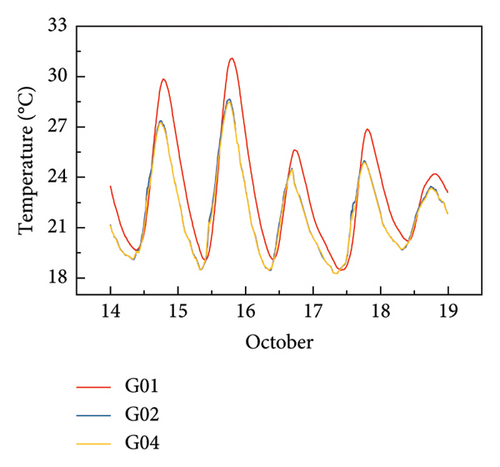
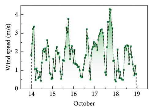
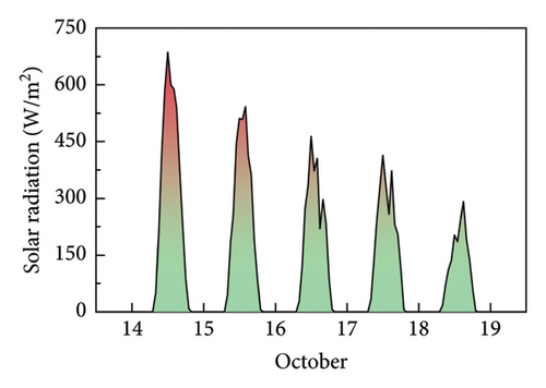
Figure 5(c) presents the variation of hourly mean wind speeds recorded by the ultrasonic anemometer in 5 days. The hourly mean wind speeds are small, ranging from 0.5 to 4.5 m/s. Owing to the absence of sensors for measuring radiative intensity in the SHM system, this study utilized hourly measurement data of solar radiation intensity from a nearby astronomical observatory located at 28.85°N, 104.97°E. Figure 5(d) illustrates the variation of hourly solar radiation intensity in the horizontal plane of the earth surface in 5 days.
4. Theory of Heat Transfer
4.1. Heat Conduction Equation
4.2. Thermal Initial Conditions and Boundary Conditions
4.3. Shadow Recognition Based on Triangle Barycenter Coordinate
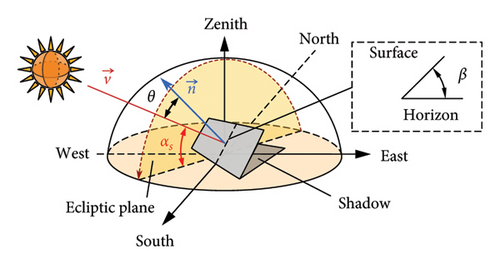
Previous studies have shown that solar radiation is a key driver of temperature gradients in a bridge [11, 28, 31–33]. Accurately determining solar shading is essential for establishing correct thermal boundary conditions. However, the mutual shading among structural components requires algorithmic identification due to its complexity and the lack of simple geometric identifiers.
The ray tracing method was first proposed by Appel in 1968 [34], and it is utilized for shadow identification with the core issue being to determine whether the emitted rays intersect with other structural surfaces [35]. The triangle centroid coordinate method is now used for such shadow analysis because of its higher computational efficiency [36, 37], and actually, it has been implemented for shadow analysis of a 220-m truss arch rib [19].
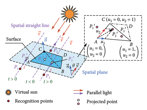
By simultaneously solving equations (11) and (12), the parameters t, u1, and u2 can be determined. Subsequently, the occlusion relationship can be determined through these parameters: occlusion occurs if and only if the equations have a solution where t > 0, u1, u2∈ [0,1], (u1+u2) ≤ 1 are concurrently satisfied, as exemplified by point P3 in Figure 8, whereas points P1 and P2 remain unobstructed.
5. Establishment of Virtual Entity
5.1. 3D FE Model for Heat Transfer Analysis
This study employs the general FE software ABAQUS [38] to construct a 3D FE model of the long-span suspension bridge, which serves as the virtual entity for temperature field analysis. Conducting heat transfer analysis at the scale of the entire bridge is highly challenging and has been rarely reported publicly. To ensure the accuracy of the 3D FE model, the geometric models of all structural components of the bridge are created in Rhino, and they are then meshed and attributed in the professional preprocessing software Hypermesh. Subsequently, custom ABAQUS-Python scripts are utilized to precisely assemble and define the remaining preprocessing parameters in ABAQUS.
The established full-bridge FE model is depicted in Figure 9. The H-shaped reinforced concrete bridge towers are modeled using solid elements. The main cables and suspenders are modeled using refined solid elements with an additional layer of shell elements on the main cable surface to simulate the wrapping band and coating. The steel wire inner core and the polyethylene (PE) sheath of the suspenders are both modeled with solid elements and assigned with distinct material properties. The main girder is modeled using shell elements to ensure multidimensional heat transfer capabilities and also consider the longitudinal and transverse slopes of the bridge deck in the geometric modeling. Notably, the bridge deck is attributed with composite shell properties, which enables the assignment of distinct material properties and thicknesses to the steel top plate of the girder and the asphalt concrete pavement, respectively. Additionally, by offsetting the neutral plane, the simulation of the actual bridge deck is achieved. This approach significantly reduces modeling complexity and computational load while accurately simulating heat transfer phenomena across layers of varying material thicknesses of the bridge deck.
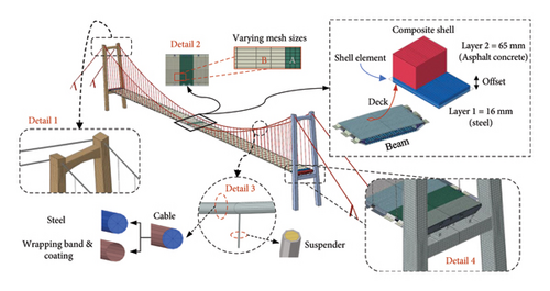
A common issue when analyzing the full-bridge model is computational efficiency. Since the main girder accounts for the majority of the mesh and nodes in the 3D FE model, variable mesh sizes are applied to the girder cross-section to reduce computational costs. Structural temperature sensors are placed on Section A of the girder, necessitating a finer mesh, while the rest of the girder sections have a relatively coarser mesh. After conducting a mesh sensitivity analysis, the seed size for the external plates of Section A is set to 0.4 m, while the external plates of the other sections are set to 1.6 m, and the internal diaphragms and wind fairings for all sections are set to 0.6 m. The final 3D FE model comprises 604,290 elements and 508,705 nodes with solid elements being DC3D8 element type and shell elements being DS4 element type.
5.2. Structural Surface Division
Considering the high computational demand of heat transfer analysis for the entire bridge, some simplifications on structural surface division are needed. The structural components of the entire bridge are divided into several regions in order to apply different boundary conditions. As shown in Figure 10, the bridge deck is divided into nine external surface regions, where the elements on the same surface region possess identical outward normal vector. The elements within the fully shaded regions are excluded from shadow recognition and considered as a single internal surface. Due to the transverse slope of the bridge deck, the east and west sides of the deck are divided separately, resulting in a total of 18 external surfaces and 2 internal surfaces for the bridge deck. The columns and crossbeams of the bridge towers are divided in a similar way. A bridge tower has 16 external surfaces and 4 internal surfaces. The main cables and hangers of the bridge are each divided into two external surfaces. Ultimately, the entire bridge is divided into (9 + 16) × 2 external surfaces and (4 + 1) × 2 internal surfaces. External surfaces undergo shadow recognition and have heat flux applied based on real-time environmental information, while internal surfaces only require heat flux based on the internal environment, reducing computational cost significantly.

5.3. Computer Programs and Virtual Entity
In addressing heat transfer issues, the precise application of thermal boundary conditions is crucial. This study utilizes the Python interface and Fortran user subroutines offered by ABAQUS to develop an automated computer program for calculating and applying thermal boundary conditions for the entire bridge. The program can automatically calculate solar parameters based on the time, date, and geographical coordinates of the bridge site, and it also identifies structural shadows in real-time. Subsequently, it calculates and imposes the thermal boundary conditions to the structural components based on the identification results and the environmental data from sensor measurements. Together with the 3D FE model, this program constitutes the virtual entity of the entire physical bridge, which will be transferred into the digital twin of the entire physical bridge for heat transfer analysis in this study and the subsequent thermal effect analysis in the future.
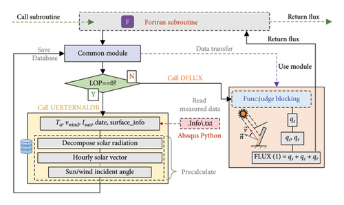
The operational principle of this program is illustrated in Figure 11. During the temperature field analysis, the Fortran subroutine is attached to the ABAQUS to participate in the computation. The Fortran subroutine is divided into three parts. The UEXTERNALDB subroutine as the first part reads external data and performs some initialization calculations with the calculated data stored in memory. Subsequently, the calculated data are passed between subroutines through “use module,” which is more advantageous for data organization and management compared to the common block method. Finally, the DFLUX subroutine is called at each analysis step, which implements shadow recognition results on the external surfaces of various structural components and calculates the solar radiation, convective heat transfer, and radiative heat transfer flux for each surface based on environmental information. The implementation of this automated computer program is detailed as follows.
5.3.1. Data Preprocessing
The positional information and normal vectors of each structural component surface, along with actual environmental data, are formatted into a readable format (.info\.txt) for the Fortran subroutine through an ABAQUS-Python script. This data set is subsequently read into the random-access memory (RAM) of the computer upon the invocation of the UEXTERNALDB subroutine. The UEXTERNALDB subroutine is called only once at the beginning of analysis by controlling the parameter LOP = 0, thereby avoiding extensive repetitive calculations and saving computational resources. The data undergo preprocessing within the UEXTERNALDB subroutine consisting of three parts.
The third part involves the prior computation of the incidence angles of solar vectors and wind directions against various structural component surfaces at different times.
5.3.2. Automated Execution of Thermal Boundary Conditions
At each step in the computational process, the DFLUX subroutine is called to calculate and apply the heat flux. Firstly, it is necessary to recognize the bridge sunshine shadow at each time in order to accurately apply solar radiation to different irradiation areas. The entire recognition process is shown in Figure 12. For the meshed surface after FE discretization, this method can be used to discriminate whether each element within the meshed surface is occluded one by one. The heat flux of solar radiation qs is then calculated based on the recognition result. The recognition program is defined as a function included in the DFLUX subroutine.
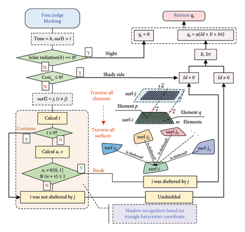
After the execution of the Fortran subroutine, the total heat flux is returned and applied as thermal boundary conditions on the structural components of the bridge.
5.4. Solution of Structural Temperature Field
In this subsection, the structural temperature field of the entire bridge on one day of October 15, 2024, is simulated using the established virtual entity and relevant measurement data through heat transfer analysis.
5.4.1. Initial Parameters
The solar radiation absorptivity coefficient α is related to the material properties, the coating on the material surface, and the degree of clear weather, and it is also affected by the rust on the steel surface and the aging of the coating. The solar radiation reflectivity re of the horizontal plane is related to the type and state of the surface. This value is generally between 0.1 and 0.8. For ordinary surfaces of the earth, it is 0.2, and for the water surface, it is 0.69 [27]. The bridge site is mainly on the water surface, so the reflectivity is initially taken as 0.69. Tables 2 and 3 summarize the parameters and the initial values of the parameters, in which Table 2 lists the parameters related to the materials and Table 3 presents the parameters related to the environment. In the following simulation, the wind speed inside the bridge girder is assumed to be zero.
| Asphalt | Steel | Concrete | PE | Coating | Unit | |
|---|---|---|---|---|---|---|
| Density (ρ) | 2.3 | 7.85 | 3.27 | 0.965 | 1.15 | kg/m3 |
| Thermal conductivity (K) | 1.8 | 55 | 3 | 0.44 | 0.032 | W/m/°C |
| Heat capacity (c) | 1,000,000 | 460,000 | 900,000 | 2,300,000 | 1,380,000 | J/kg/°C |
| Emissivity coefficient (ε) | 0.92 | 0.685 | 0.65 | 0.88 | 0.93 | — |
| Absorptivity coefficient (α) | 0.6 | 0.4 | 0.85 | 0.65 | 0.63 | — |
| Inside girder | Outside girder | |
|---|---|---|
| Convective heat transfer coefficient A (hcA) | 6 | 6 |
| Convective heat transfer coefficient B (hcB) | — | 4 |
| Reflected coefficient (re) | 0.69 | |
5.4.2. Initial Conditions
Prior to the analysis, the initial temperature field for various structural components must be determined. To eliminate the impact of uncertainties in the initial temperature field on the simulation results, a series of preanalyses of different durations are conducted to find a stable initial temperature field. A uniform temperature of 20°C is set to all the components of the bridge at the beginning of each preanalysis. As shown in Figure 13, when the duration of preanalysis is 24 h, the temperature variations at three measurement points are all less than 0.2%, indicating that the initial structural temperature field is stabilized.
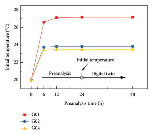
Therefore, the measurement data on October 14, 2024, are used to conduct a 24 h preanalysis. The resulting temperature field from the preanalysis is then imported as the initial conditions for the heat transfer analysis on October 15, 2024. This way is adopted in order to mitigate the impact of uncertainties in the initial temperature field.
5.4.3. Results and Analysis
Considering both computational time and accuracy, a heat transfer analysis is performed every hour for a total of 24 h. In ABAQUS, the Fourier heat conduction equation is solved for each structural component under prescribed thermal boundary conditions, employing the variational formulation principle and the standard Galerkin method, thereby obtaining the 3D structural temperature field of the entire bridge.
Figure 14 shows the comparison of the simulated results with the measured temperature values at the sensor locations. From the comparison, it is observed that the simulated temperature values share the same trend as the measured values, both exhibiting cyclical changes in structural temperature throughout the day. For the sensor G01 inside the girder, the simulated temperature values are slightly lower than the measured values. For the bottom plate at the sensors (G02 and G04), the temperature difference between the measurement and simulation appears mainly from 8:00 to 18:00 during the daytime, in which solar radiation exists. At night without solar radiation (18:00 to 8:00), the simulated temperature values are close to the measured temperature values. This suggests that the complex effects of solar radiation together with highly uncertain model parameters make it difficult to obtain accurate temperature values during the daytime. This also indicates that the differences between the simulated and measured temperatures are caused by inaccurate model parameters.
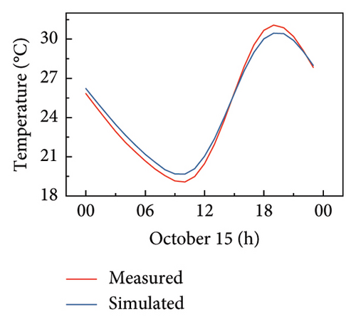
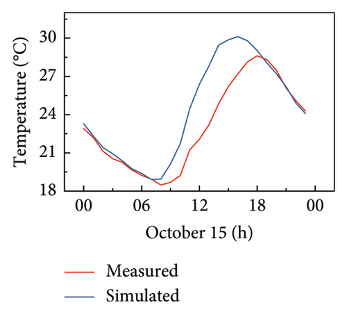
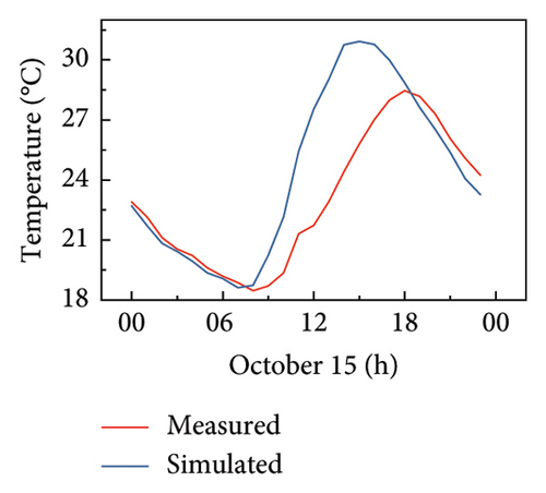
In summary, the convective heat transfer inside the girder is slightly underestimated and the solar radiation intensity is inaccurately estimated in the simulation. This is attributed to the high uncertainties of the initial parameters selected, which do not reflect the bridge site environment. Therefore, digital twin technology needs to be employed to address this issue.
6. Model Updating of Virtual Entity for a Digital Twin
6.1. Objective Function and Updated Parameters
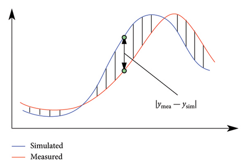
The selection of updated parameters needs to fully consider all the parameters that may affect the accuracy of the simulation results of the virtual entity. The parameters influencing the simulation results include not only the thermal parameters of the materials but also the empirical coefficients when simulating the thermal boundary. As discussed in Section 4, the factors influencing the thermal boundary mainly include convective heat transfer, radiant heat transfer, and solar radiation. The inaccurate approximation of these parameters may lead to significant errors in the simulated temperature distribution.
| Parameter | Sensitivity |
|---|---|
| Density(ρ) of asphalt | |Si| < 1 × 10⁻⁴ |
| Thermal conductivity(K) of asphalt | |Si| < 1 × 10⁻⁴ |
| Heat capacity (c) of asphalt | |Si| < 1 × 10⁻⁴ |
| Emissivity coefficient (ε) of asphalt | |Si| < 1 × 10⁻⁴ |
| Absorptivity coefficient (α) of asphalt | 0.057 |
| hcA outside girder | −0.020 |
| hcB outside girder | −0.016 |
| Density (ρ) of steel | |Si| < 1 × 10⁻⁴ |
| Thermal conductivity (K) of steel | |Si| < 1 × 10⁻⁴ |
| Heat capacity (c) of steel | |Si| < 1 × 10⁻⁴ |
| Emissivity coefficient (ε) of steel | −0.013 |
| Absorptivity coefficient(α) of steel | 0.015 |
| hcA inside girder | −0.012 |
| Reflectivity re | 0.044 |
The results of the sensitivity analysis are presented in Table 4, and based on these results, the parameters ultimately selected as updated parameters are α of asphalt, α of steel, ε of steel, hcA outside girder, hcB outside girder, hcA inside girder, and reflectivity re.
6.2. PSO Algorithm
Using an intelligent optimization algorithm for updating [44–46] to gradually establish the mapping relationship between the physical entity and its virtual counterpart while minimizing the assumptions involved in simulations is a crucial step in constructing a digital twin. This study adopts the PSO algorithm to update the selected parameters. The PSO algorithm is capable of adjusting the parameters based on real-time sensor data to accommodate real environmental conditions and reduce the uncertainties in the selected parameters.
The PSO algorithm [47] is an optimization technique based on swarm intelligence, simulating the foraging behavior of bird flocks. In PSO, each solution is regarded as a “particle” in the search space. The particles adjust their flight paths based on their own experience and group experience to find the optimal solution. Each particle has two attributes: position and velocity, representing the current solution and the moving trend toward the optimal solution. The particles update their positions and velocities during the iteration process. The velocity determines the search direction and step size of the particles. The particles adjust their velocities and positions based on their own historical best position (individual experience) and the best position in the entire group (group experience). In this way, the PSO algorithm can find the approximate optimal solution of the problem in the complex search space.
6.3. Virtual Entity Updating
The computational framework for the updating process is depicted in Figure 16 with the entire procedure executed in an external Python environment.
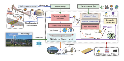
The PSO algorithm, written in the external Python, generates updated parameter files for Fortran subroutines and ABAQUS input files during each iteration. Subsequently, batch computations are conducted by invoking ABAQUS through CMD commands scripted in the external Python, facilitating parallel processing of multiple models and accelerating the computational speed. Finally, the external Python automatically calls ABAQUS built-in Python to extract the results, calculate the objective functions, and complete iterations. The measurement data recorded on October 15, 2024, are selected to simulate the thermal boundary conditions and establish the digital twin.
6.4. Digital Twin Establishment
Utilizing 5 particles in the iteration process and after 21 iterations, the change in the target value between two consecutive iterations becomes less than 5%, leading to the termination of the iteration process, with the final iteration time being 10 h and 27 min. Figure 17 illustrates the variation of the objective function during the updating process. This computational process is conducted on the 32 cores of the AMD Ryzen Threadripper 3970X processor.
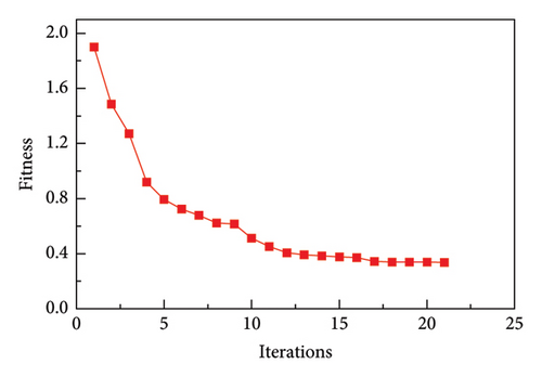
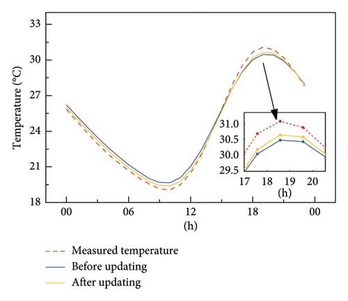
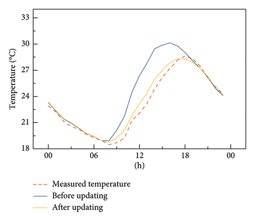
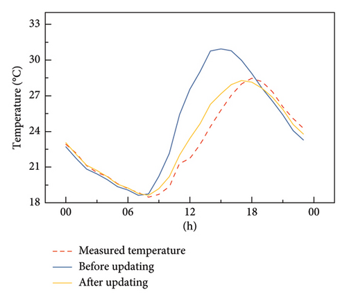
Figure 18 compares the simulation results before and after updating together with measured structural temperature results. Table 5 summarizes the changes in the parameters before and after updating. After updating, the average temperature difference across all the sensors is 0.31°C, a significant improvement compared to the initial difference of 1.89°C. It is noted that there are still minor discrepancies between the measurement and digital twin results of the structural temperatures at sensors G02 and G04. Since these discrepancies primarily occur during daytime (approximately 6:00 AM to 6:00 PM), it is inferred that the cause of these discrepancies is mainly due to the inaccuracy in solar radiation measurement. The solar radiation measurement data used in this study are sourced from a meteorological station other than the bridge site, and it represents an average value for the region. The actual solar radiation received by the bridge may deviate from it, dependent on the cloud cover of the bridge.
| No. | Updating parameters | Initial values | After updating | Difference (%) |
|---|---|---|---|---|
| 1 | α of asphalt | 0.60 | 0.51 | −15.00 |
| 2 | α of steel | 0.40 | 0.27 | −32.50 |
| 3 | ε of steel | 0.69 | 0.80 | +16.79 |
| 4 | hcA outside girder | 6.00 | 5.20 | −13.33 |
| 5 | hcB outside girder | 4.00 | 3.41 | −14.75 |
| 6 | hcA inside girder | 6.00 | 7.81 | +30.17 |
| 7 | re | 0.69 | 0.31 | −55.07 |
It is seen from the updated parameters that the absorptivity coefficients for asphalt and steel, as well as the reflectivity of the water surface, all decrease to varying degrees. Notably, the reflectivity of the water surface decreases by 55.07% because of the presence of a sandbar in the center of the river, indicating that using a reflectivity coefficient of 0.69 for the water surface does not accurately reflect the actual environmental conditions. The initial parameters overestimate the role of solar radiation, leading to an overestimation of temperatures at the two sensors, G02 and G04, located at the bottom slab during the daytime. Similarly, the convective heat transfer coefficient outside the box girder decreases after updating, while that inside increases, indicating that the initial parameters overestimate the convective heat transfer effect outside the box girder and underestimate the effect inside due to uncertainties in wind speed.
7. Prediction of Structural Temperature Field by Digital Twin
7.1. Prediction of Structural Temperature at Measurement Points
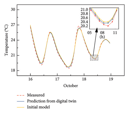
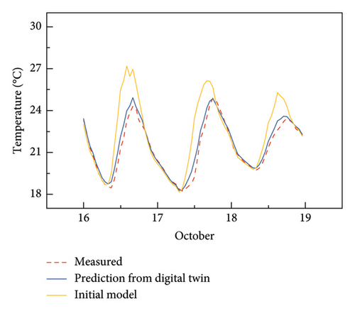
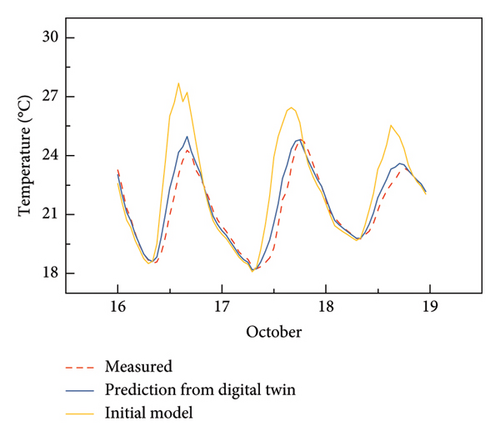
To demonstrate the prediction capacity of the established digital twin with updated parameters, the environmental data of the next 3 days from October 16 to 18, 2024, are used as input data to the established digital twin to calculate the structural temperature at the sensors. Figure 19 shows the comparison results of structural temperature among the measured values, the predicted values, and the values given by the virtual entity with initial parameters. The comparison results clearly show that the digital twin can well predict the structural temperature of the bridge at the sensor locations. The average temperature difference between the simulation by the digital twin and the measurement is approximately 0.27°C, while the maximum temperature difference is 1.2°C. In contrast, the average temperature difference between the simulation by the virtual entity with initial parameters is approximately 0.86°C, while the maximum temperature difference is 5.05°C. The comparison results also show that the simulation results by the digital twin at night are better than those during the daytime. The average temperature difference at night is approximately 0.1°C, and the average temperature difference during the daytime is approximately 0.5°C. This may be because the solar radiation data provided by the meteorological station represent the average value of an area and are different from the solar radiation actually received by the bridge.
7.2. Prediction of Structural Temperature Field of Entire Bridge
Due to the limited number of structural temperature sensors installed on the bridge, the temperature of most structural components is often unknown. Nevertheless, by using the established digital twin, the structural temperature field of the entire bridge can be predicted.
7.2.1. Temperature Distribution of Bridge Deck
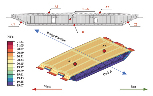
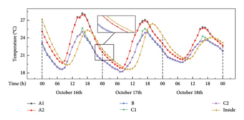
Figure 20 shows the structural temperature values at six points of Section A of the bridge deck. Section A is the midspan of the bridge deck, and there are no sensors at the six points. It is seen that the maximum temperature of the top slab can reach 28°C, occurring between 14:00 and 16:00 in the afternoon, with a variation of approximately 10°C during a day. Due to the effect of solar radiation, the temperature of the top slab is higher than that of the bottom slab, and the maximum temperature difference can reach 3.4°C. With the rise and set of the sun and considering the cross slope of the top slab, the maximum temperature at Point A1 on the west side is approximately 0.4°C greater than that at Point A2 on the east side. The temperature change of the inner plate of the box girder shows a time delay, that is, the times when the maximum and minimum temperatures occur inside the girder are 1 to 2 h later than those of the top slab. Furthermore, the temperature inside the box girder is higher than that at the top and bottom surface of the box girder during night because of the slow heat transfer.
It is noteworthy that the calculated horizontal temperature difference in the steel box girder is not significant. This is related to the orientation of the bridge investigated in this study. As shown in Figure 2, the bridge is primarily oriented in the east–west direction. Since the sun moves from the east to the west, the two symmetric sides of the bridge deck with respect to its longitudinal axis receive nearly equal amounts of solar radiation at the same time.
Figure 21 shows the temperature change of the two points on the east and west sides of the top plate of the girder along the longitudinal direction of the bridge in one day. It is seen that even though the longitudinal slope of the bridge deck is considered in the modeling of the girder, the temperature difference between the east and west sides of the top plate is insignificant. This is because the longitudinal slope of the deck is small, and the normal vectors of the longitudinal plate of the bridge deck on both sides are close so that the received solar radiation is similar.
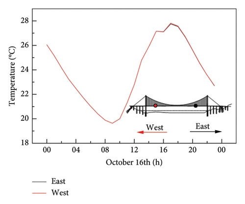
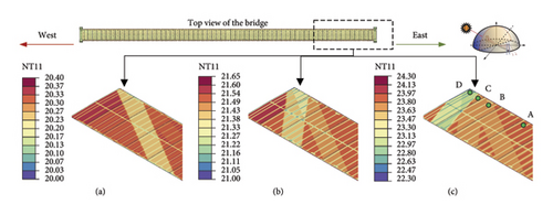
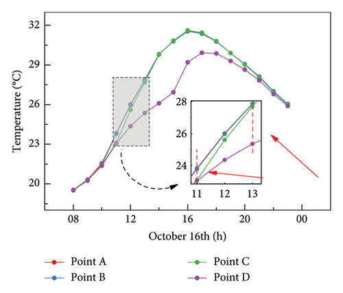
Figure 22 shows the locations of the four Points A, B, C, and D on the top plate of the girder at different distances from the tower on the east. Figure 23 shows the temperature changes at the four points in 16 h. Among the four points, Point A has no shading, while Points B, C, and D are shaded by the tower at different times. Since Point B is shaded at 10:00 AM when the solar radiation intensity is small and the shadow disappears quickly, the temperatures of Points A and B do not differ much. Point C is shaded by the tower between 10:00 and 11:00 AM, during which the temperature is the same as that of Point D. After 11:00 AM, Point C is exposed to solar radiation. Consequently, the temperature of Point C rapidly rises after 11:00 AM and becomes close to that of Point A. Point D is shaded by the tower for the longest time. Therefore, its temperature is lower than that of Point A. The maximum temperature difference can reach 3.8°C. After nightfall, the temperatures of Points A, B, C, and D converge and become closer.
7.2.2. Temperature Distribution of Bridge Tower
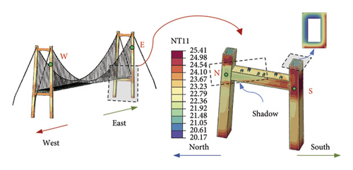
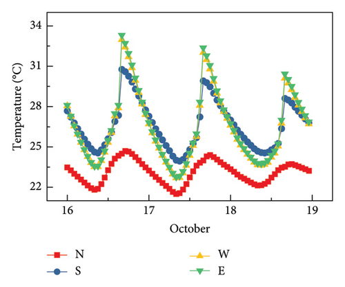
Figure 24 shows two points W and E on the upper columns of the two towers at the same height and two points N and S on the north and south columns near the lower crossbeam of the east tower. Figure 25 displays the temperature changes at the four points within 3 days. Since the upper columns are not shaded and the orientations of the surfaces, where points W and E are located, are the same, the temperature changes at the two points do not differ much. The tower columns near the lower crossbeam are prone to being shaded by the girder. Compared with the unshaded side, the maximum temperature difference on the shaded side can reach 5°C, indicating that solar radiation is the main reason for the uneven temperature.
7.2.3. Temperature Distribution of Main Cable
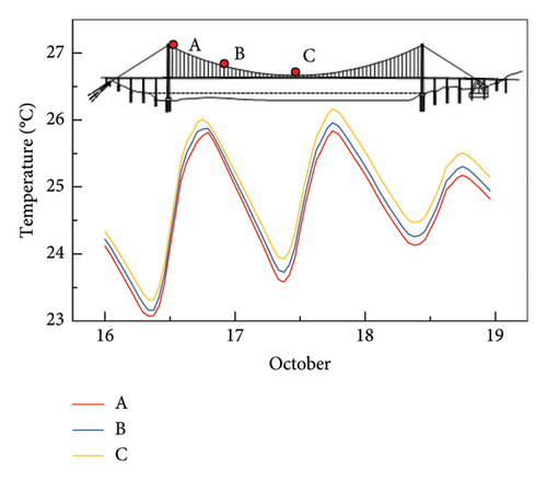
The comparison of temperature changes at three Points A, B, and C of the center of the main cable within the 3 days is shown in Figure 26. The results indicate that as the height above the river increases, wind speed gradually increases, leading to more significant convective heat transfer effects and lower temperatures.
8. Concluding Remarks
- 1.
It is feasible to develop a digital twin for predicting the structural temperature field of a long-span suspension bridge by mapping the measurement data with the virtual model of the bridge through the PSO algorithm.
- 2.
It is necessary to develop an automated computer program to determine complex thermal boundary conditions and calculate 3D structural temperature field of the entire bridge through a secondary development of combination usage of several commercial software.
- 3.
The developed digital twin can consider the mutual shading effect and solar radiation of structural components of the entire bridge and minimize the uncertainties in the conventional temperature simulation, thereby obtaining more precise simulation results.
- 4.
The digital twin can be used to predict the current temperature distribution of all the structural components of the long-span suspension bridge once it is established. Compared to the conventional simulation model with initial parameters, the digital twin can reduce the average temperature difference to 0.3°C, indicating a higher accuracy of prediction.
- 5.
The developed digital twin can be used to predict the future temperature distribution of all the structural components of the long-span suspension bridge if the future environmental conditions of the bridge are given. The results show that nonuniform temperature distributions of a long-span suspension bridge in space occur mainly due to nonuniform solar radiation and mutual shading effect on the structural components of the bridge.
Nevertheless, it is noted that the number of temperature sensors installed on the bridge is limited and there are no temperature sensors installed on the bridge towers and main cables. The solar radiation data obtained from the meteorological station represent regional averages, which may not accurately reflect the actual solar radiation of the bridge site. Given these limitations, it is recommended that additional structural temperature sensors and pyranometers should be installed on the bridge to enhance the accuracy of the digital twin established. Furthermore, it is desirable to apply the proposed framework and computer program to other bridges once the chance is available to the authors in the future. The structural temperature field of the entire bridge determined by the digital twin in this study will be imported into ABAQUS for subsequent thermal analysis of the entire bridge with the updated FE model in the future.
Conflicts of Interest
The authors declare no conflicts of interest.
Author Contributions
Ning-Jie Zhou: investigation, methodology, software, formal analysis, visualization, data curation, and writing – original draft. Ning-Jie Zhou: conceptualization, investigation, methodology, funding acquisition, supervision, and writing – review and editing. Zi-Jing Wei: investigation and data processing. Di Wu: investigation and data curation. Er-Hua Zhang: investigation and data curation.
Funding
The works described in this paper are financially supported by the Changjiang Scholars Program of the Ministry of Education of China (SWJTU-WB0100111012209) to which the authors are most grateful.
Acknowledgments
The works described in this paper are financially supported by the Changjiang Scholars Program of the Ministry of Education of China (SWJTU-WB0100111012209) to which the authors are most grateful.
Open Research
Data Availability Statement
The data used to support the findings of this study are available from the corresponding author upon request.


